

Results and Discussion
Using the Langmuir Isotherm Model to Calculate the Total Binding Capacity of Hydrocarbon2 (HC2)
Solutions of basic blue 3 dye (BB3) and, independently, fluorescein disodium (FL) in 35 ppt salinity salt water were prepared by adding 30 mg of dye to 1.20 L of salt water (from Instant Ocean salt mix and distilled water, 77 oF). 100.0 mL portions of each dye solution were placed in 250 mL flasks, and so each flask initially contained 2.5 mg of dye and the overall dye concentration was 25 mg/L. A carefully weighed amount of HC2 was added to each flask. The amounts added ranged between 10 mg and 100 mg as indicated in Table 1. Each flask was tightly stoppered and clamped onto a shaker apparatus that continuously agitated the flasks to ensure good contact between the solution and the HC2 sample. The dye concentration in each flask was assayed every 3 – 5 days by spectrophotometric measurement using a Beckman DU70 Spectrophotometer. The BB3 sample dye concentrations were measured at 645 nm, and the fluorescein solutions were recorded at 490 nm (nm = nanometer, a measure of spectral wavelength). The experiment was continued until sequential measurements did not exhibit much change in the amount of dye present (i.e. the HC2 was saturated and could not absorb any more dye). This criterion was met in the BB3 run at 17 days, whereas the fluorescein samples reached equilibrium after 14 days. The experimentally measured dye absorptions are given in Table 1. The key Langmuir model parameters 1/x and 1/C (Eq. (5)) can be derived from these experimental quantities (Table 1). 1/C is just the inverse of the dye concentration at the end of the experiment (= equilibrium), and this dye concentration can be derived by simply multiplying the initial dye concentration (= 25 mg/L) by the ratio Aeq/A0, where Aeq and A0 are the dye absorptions of the solution at the end of the experiment and at the beginning, respectively. The quantity 1/x is calculated by dividing the amount of HC2 used by the amount of dye absorbed (= (2.5 mg)(1-Aeq/Ao)). Graphing 1/c vs. 1/x then gives the desired quantity, the binding capacity (xm) of HC2 for these dyes, as the inverse of the Y-intercept. By this analysis, HC2’s binding capacity for BB3 in seawater is 61 ± 7 mg/gm, and for fluorescein is 45 ± 2 mg/gm. Note that the Y-intercept values from Figure 3 are reported in units of mg of HC2/mg of dye, so the derived xm value was multiplied by 0.001 to arrive at the mg of dye/gm of HC2 values noted above. For subsequent analyses, it will become convenient to just average these values to derive a “general” binding capacity for dyes by HC2; xm(ave) ~ 53 mg/gm.
| HC2 (mg) | A0 | Aeq | 1/C (L/mg) | 1/x (mg HC2/mg dye absorbed) |
|---|---|---|---|---|
| 0 | 2.77 | |||
| 20.1 | 1.56 | 0.071 | 18 | |
| 39.8 | 0.39 | 0.28 | 19 | |
| 60.1 | 0.32 | 0.35 | 27 | |
| 100.4 | 0.090 | 1.20 | 42 | |
| 0 | 2.30 | |||
| 10.4 | 1.90 | 0.048 | 24 | |
| 41.3 | 0.98 | 0.094 | 29 | |
| 100.7 | 0.24 | 0.38 | 45 |
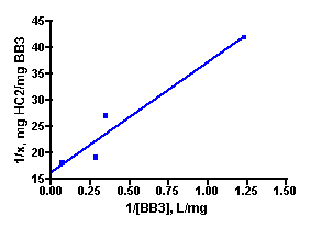
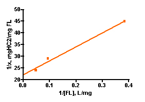
Figure 3. Graphical representation of the Langmuir isotherm experiment. BB3 is on the top (r2 = 0.94), and fluorescein is on the bottom (r2 = 0.99).
Rate of Dye Removal as a Function of HC2 Amount
The first series of dye removal experiments utilized constant amounts of both BB3 and fluorescein, and the amount of GAC was varied. We expected that the calculated k values would be invariant with respect to the amount of GAC used (see the discussion associated with Eq. (3)), and so these experiments will provide a good test of our model and its assumptions. The experimental set-up is simple, and follows one used by other authors. A five-gallon bucket with a small aperture in the top was filled with 4.0 gallons of freshly prepared 35 ppt salinity salt water, and 243 mg of basic blue 3 (7) and 268 mg of fluorescein disodium (8) were added (16 and 18 ppm, respectively). These two dyes were run simultaneously since their spectral signatures do not overlap. The Phosban reactor was charged with the indicated amount of pre-washed Hydrocarbon2 GAC (see Table 2), and an Eheim1048 pump was used to remove water from the bucket, push it through the Phosban reactor, and then return it to the bucket in a closed loop arrangement. The pump was adjusted to a flow rate of 49 gph (0.81 gpm). Samples of the reservoir water were removed at specific time intervals, typically every 5 – 15 min over a 120 – 180 min time course, and these samples were assayed for dye content with the Beckman DU70 UV/VIS spectrophotometer. As with the Langmuir isotherm experiments, the blue dye signal was monitored at 645 nm, and the fluorescein signal was monitored at 490 nm. No effort was made to adjust the solution temperature, which typically increased from 72 to 75 oF during the run. If the GAC column in the Phosban reactor began to separate due to the vigorous water flow, the cylinder was gently tapped until the GAC particles repacked into a single column. Control experiments (dye + salt water/no GAC) demonstrated that the dyes did not decompose over the experimental time regime.
Figure 4 below shows the amount of dye remaining (as the quantity ([dye]t/[dye]0)) as time progresses for five different amounts of HC2: 25 gm, 50 gm, 75 gm, 100 gm, 150 gm, and 200 gm. Each individual experiment was replicated 2-3 times, but only a single representative data set is shown on the graphs for simplicity of presentation. These HC2 amounts span a range from about 6 to 50 gm/gal, and correspond to filling the Phosban reactor from 0.8″ to 6.5″ in height with the Hydrocarbon2. Some useful interconversions are:
(16) Grams of HC2 = 31 • height of the HC2 column, in inches
(17) Grams of HC2 = 81 • cups of the HC2
Inspection of the graphs indicate that indeed, the amount of blue dye (left) and fluorescein (right) remaining decreases over time, and that the rate at which the amounts decrease depends on the amount of GAC present. The mathematic treatment derived in Eq. (13) can be used to process these raw data into the desired quantity, k, the rate constant for dye removal (Table 2). Since both BB3 and fluorescein were run together, we can only report an averaged rate constant for them both. This simplification is in line with the expectation that in an aquarium setting, the DOC that GAC removes is quite heterogeneous, and average values for a compilation of compounds are probably more valuable than the rate constant value for any particular compound. The rate constants shown in Table 2 are the average values from the 2-3 independent runs for each set of unique experiments. In addition, the r2 values for the data are given; these numbers reflect how accurately the mathematical model fits the data. Any value of r2 greater 0.9 is good, and any r2 values over 0.98 indicated an exceptionally solid correlation between the model and the data.
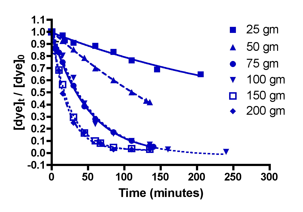
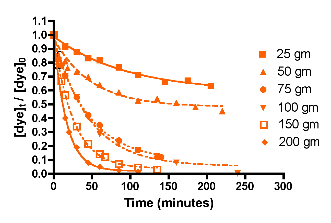
Figure 4. Basic Blue 3 (7) (top) and fluorescein (8) (bottom) removal by Hydrocarbon2 GAC as a function of GAC amount.
| Amount of HC2, gms | |||||||
|---|---|---|---|---|---|---|---|
| 25 | 50 | 75 | 100 | 150 | 200 | ||
| Basic Blue 3 andFluorescein | k (L/mol-min) | 9.6 ± 0.6 | 13 ± 0.7 | 27 ± 0.5 | 21 ± 1 | 31 +2 | 28 ± 1 |
| r2 | 0.97 | 0.99 | 0.99 | 0.98 | 0.98 | 0.99 | |
| t90 (hr) | 22 | 7.1 | 2.2 | 2.2 | 0.99 | 0.81 | |
As discussed earlier, all of the calculated k’s should be identical, since k is independent of the amount of GAC present. The fact that they are not requires some interpretation. The rate constant values for each dye when GAC ≥ 75 gm do indeed approach this criterion, lending confidence to the mathematical model for GAC-based dye removal in this GAC range. However, the rate constants k for the 25 and 50 gm of GAC runs are anomalously small. A possible explanation for this discrepancy emerges upon consideration of the actual manner in which the GAC packs into a bed in the Phosban reactor. It is possible, for example, that at the low HC2 loadings (25 and 50 gms), the shallowness of the GAC bed (< 1″ for the 25 gm runs) allows channeling of the current, which in turn leads to GAC dead spots and diminished opportunities for dye binding. As the GAC amount increases, the bed becomes thicker, channeling is reduced, and more of the GAC charge can be utilized in dye binding. In this scenario, the higher loadings of HC2, which correspond to the more realistic GAC bed depths of 2.5 – 6.5″, operate normally, and would fall under the purview of a typical Phosban charge in an aquarium setting. The k values between 75 and 200 gms of HC2 vary from 21 to 31 L/mol-min, a spread of about 20% (ave = 26 ± 5 L/mol-min). Given the assumptions used and all of the other possible experimental variables, this level of variation is not very surprising, and it is a reminder that we will likely only be able to draw approximate and not numerically precise conclusions from this analysis. However, one early conclusion can be drawn from these data: using less that 75 gm of GAC (< 2.5 inches) in a Phosban reactor is not an effective way to utilize GAC for impurity removal.
The time required to remove 90% of the dye (t90, see Eq. (14) and the accompanying discussion) can be calculated for these experiments as well, see Table 2. These t90 values are specific to the conditions of the dye removal experiment (i.e., functions of flow rate and volume, mass of HC2, and the starting dye concentration). By plotting the t90 values as a function of the amount of HC2, the complex relationship between the quantity of HC2 and the rate of dye removal is revealed. These data are presented in Figure 5. It is apparent from inspection of Figure 5 that once a charge of 75 gm of HC2 (or greater) is used, the t90 values do not change much. Since the t90 values are a function of the rate constant k, and k does not change much in this HC2 range, this observation is not surprising. One interpretation of this trend is that when HC2 amounts above the 75 gm threshold are used, a large excess of HC2 binding sites are available compared to the amount of dye present, and so the dye molecules always “see” binding sites. This hypothesis is buttressed by the fact that 511 mg of dye in total is used in each experiment, and with an average binding capacity of 53 mgs of dye per gram of HC2 (from the calculated xm above), only about 10 grams of HC2, in principle, is required to sop up all of the dye. Of course, since there is a great heterogeneity of binding sites, it would take a long time (recall the Langmuir binding experiments took over 14 days to reach equilibrium) to saturate all of the slow-binding sites. And so, it appears empirically that in the region above 75 grams of HC2, there are enough fast-binding sites to absorb the dye over the course of the 2-3 hour experiment. It is likely that in an aquarium, the fast binding sites are responsible for most of the absorption as well.
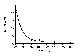
Figure 5. t90 values for dye removal as a function of the amount of HC2 used.
Rate of Dye Removal as a Function of Dye Structure and of Flow Rate
The next series of experiments probed two independent questions:
- How does the chemical structure of the dye molecule influence its rate of removal by HC2?
- How do dye removal rates respond to changes in the flow rate through the Phosban reactor?
The first question was examined by choosing one arbitrary set of experimental parameters (flow = 49 gph, 100 gm of Hydrocarbon2, 15-21 ppm of each dye molecule in a volume of 4 gallons) and measuring the decrease in dye absorption for the four dyes chosen, Basic Blue 3 (7) and Fluorescein (8) combined, Acid Yellow 76 (9) and Chlorophyllin (10). The choice of a 100 gram Hydrocarbon2 charge should put these experiments in the “constant k” regime of dye removal (cf. Table 2) where channeling through the GAC is not important. The Basic Blue 3 and Fluorescein 100 gm Hydrocarbon2 results are already described in Section 2.2. The remaining two dyes, 9 and 10, were run separately since there was insufficient spectral dispersion to make meaningful measurements in mixtures. In addition, both 9 and 10 were not soluble at the 15 ppm level in 35 ppt salt water. Therefore, these two dyes were examined in pure distilled water. This change in media raises obvious concerns about the relevance of the data acquired to questions of reef tank DOC removal. In order to address these concerns, a mixture of Basic Blue 3 (15.9 ppm) and Fluorescein (17.5 ppm) in pure distilled water was subjected to a HC2 removal run at 72 gph with 50 gm of HC2 (this issue was probed before we realized the benefits of using an HC2 amount greater than 75 gms). The measured rate constant for dye removal under these circumstances (k = 5.7 ± 0.3 L/mol-min) does differ from the same values obtained in salt water under identical experimental conditions (k = 4.1 ± 0.2 L/mol-min), and so some caution is necessary in interpreting the dye-to-dye comparison data. However, the discrepancy is not large, and so it will not affect the overall tenor of the conclusions.
A second independent series of dye removal experiments was conducted at a higher flow rate, 72 gph. These flow rate values (49 and 72 gph) span the range of suggested flow rates supplied with the Phosban reactor. The data are presented in Figure 6 and Table 3.
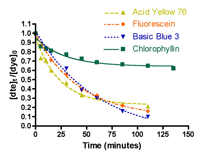
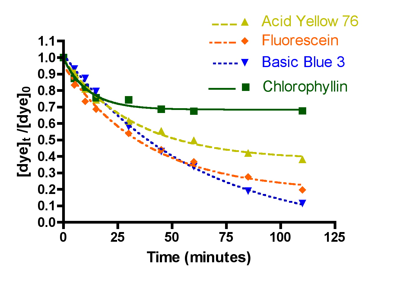
Figure 6. Basic Blue 3, Fluorescein, Acid Yellow 76 and chlorophyllin removal as a function of time. Top: 49 gph.; Bottom: 72 gph. (100 gms of Hydrocarbon2, 15-21 ppm dye each).
| dye | flow rate (gph) | ||
|---|---|---|---|
| 49 | 72 | ||
| Basic Blue 3 andFluorescein | k (L/mol-min) | 21 ± 1 | 18.0 ± 0.3 |
| r2 | 0.98 | 0.99 | |
| t90 (hours) | 2.2 | 2.4 | |
| Acid Yellow 76 | k (L/mol-min) | 14.1 ± 0.6 | 7.7 ± 1 |
| r2 | 0.97 | 0.92 | |
| t90 (hours) | 3.0 | 5.4 | |
| Chlorophyllin | k (L/mol-min) | 2.6 ± 0.3 | 2.1 ± .4 |
| r2 | 0.94 | 0.80 | |
| t90 (hours) | 16 | 20 | |
The question of dye removal rate as a function of dye structure can be addressed in a general sense by considering the graphs depicted in Figure 7. It is clear from inspection of these graphs that the rate of dye removal does vary as per the dye structure. This variation can be quantified by application of Eq. (13) as described in the Mathematical Modeling section, and the values of the derived rate constants are presented in Table 3. The differences in rates of removal are not large, however, and vary no more that a factor of 10 between fastest (Basic Blue 3/Fluorescein) and slowest (Chlorophyllin).
The experimental observation that the rate constants for dye removal, k, decreased at the faster flow with all of the dyes was unexpected. Intuitively, an increase in the rate constant for dye removal might be expected to result from a situation in which more dye-containing solution passes through the GAC bed per unit time (i.e., faster flow rate). How can this discrepancy be rationalized? In fact, it is typical for flow-through reactor experiments such as the one used in these studies to find that mass transfer of the solute (= dye molecules in this case) from the bulk solution to the adsorption site is actually the slow, or rate-limiting, step. Since the rate constant can be thought of as a probability of adsorption as the solution passes through the GAC layer, the residence time of a given dye molecule becomes important. If the residence time is long compared with the time it takes for the dye molecule to find its adsorption site, then the k value will be high. On the other hand, if the residence time is short compared to the time it takes for the dye to find its adsorption site, then the k value will be smaller. Residence time scales inversely with flow rate, so it is possible that we have entered a regime where the faster flow (= less residence time) lead to lower k’s. Some experimental evidence that supports this conclusion can be found in Figure 7, where the k values scale inversely with the molecular weight of the dyes. This behavior is consistent with a scenario where mass transfer in solution, which also scales inversely with increasing molecular weight, is a significant factor in the overall kinetics. That is, the more a molecule weighs, the slower is its transit from point A to point B in solution, and so it benefits (= larger k) from a longer residence time in the GAC bed (= slower flow rate).
Is it possible to delve deeper into these rate vs. structure differences and arrive at some correlation between the rate constant for dye removal and some measurable molecular parameter? If such a relationship can be discerned, then these model dye experiments may have some predictive value in terms of removal efficiencies for the types of compounds that have been proposed as components of DOC in the marine environment. We examined the correlation between dye removal rate constants k and three molecular parameters: molecular weight, molecular volume, and molecular surface area of the dye. The former value is just the sum of the weights of the component atoms. The latter two values were calculated by using a commercially available computational chemistry program called Spartan [Spartan’04], one of the standard tools of chemists who work with complex organic molecules. The data are plotted in Figure 8. As can be seen by inspection of these graphs, there is significant correlation between each of the molecular parameters and the rate constant for dye removal, k. Perhaps a larger data set of structurally different dyes might have yielded even more compelling relationships, but at the very least, there does appear to be a trend among these data sets: molecules with smaller molecular weights/volumes/surface areas appear to be removed faster by HC2. Thus, GAC might be better at removing the smaller molecular metabolites, colored or uncolored, that are inevitably produced in marine tanks compared to the larger biomacromolecules (or large fragments thereof), such as proteins, polynucleic acids, and oligosaccharides that also are present. As discussed earlier, this k dependence on size may be largely attributed to the inverse relationship between molecular weight and mass transfer in solution.
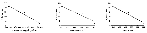
Figure 7. Rate constant, k, for the different dyes vs. measurable molecular parameters.
Leaching Experiments: Does Saturated GAC Release Bound Dyes?
How well do the dyes stick to the GAC particles? Do the dyes (and by inference, DOC’s) leach back out into solution over time? Actually, just such leaching in the context of equilibrium binding is a requirement for application of the Langmuir isotherm model to measuring dye saturation points. In the context of aquarium chemistry, this concern becomes particularly relevant if the GAC in an aquarium setting is not changed out prior to saturating. At that point, will it serve as a DOC source, slowly polluting the aquarium water?
This question was examined by recovering the used HC2 from Chlorophyllin and Basic Blue 3 adsorption experiments, washing it with distilled water, and then resuspending it in the Phosban reactor. Distilled water was added to the reservoir and the Phosban reactor in the usual amounts (4.0 gallons), and the Eheim pump was turned on to 49 gph. The dye content of the reservoir was measured at the indicated time intervals (Figure 8). For these experiments, the [dye]o measurement was taken a few minutes after adding the dye-saturated HC2 to the pure water. Therefore, the [dye]t/[dye]o ratio should increase over time, as more dye diffuses out of the HC2. From these data, it appears that both Chlorophyllin and Basic Blue 3 leach out in observable and significant quantities over the course of several hours. The Chlorophyllin concentration ultimately diminishes, but based upon the color changes observed at long experimental times, it is possible that this species is undergoing some type of chemical destruction (oxidation? demetalation of the porphyrin core?) in competition with HC2 binding. Extrapolating from these dye results to DOC in the aquarium requires the usual caveats, of course, but these observations are suggestive of the fact that organics may not stay stuck to GAC over time. This tentative conclusion raises the concern that keeping saturated, or spent, GAC in the system past its useful life may be problematic. Is there a way to “guestimate” when the GAC is saturated? Section 3.2 will address this point.
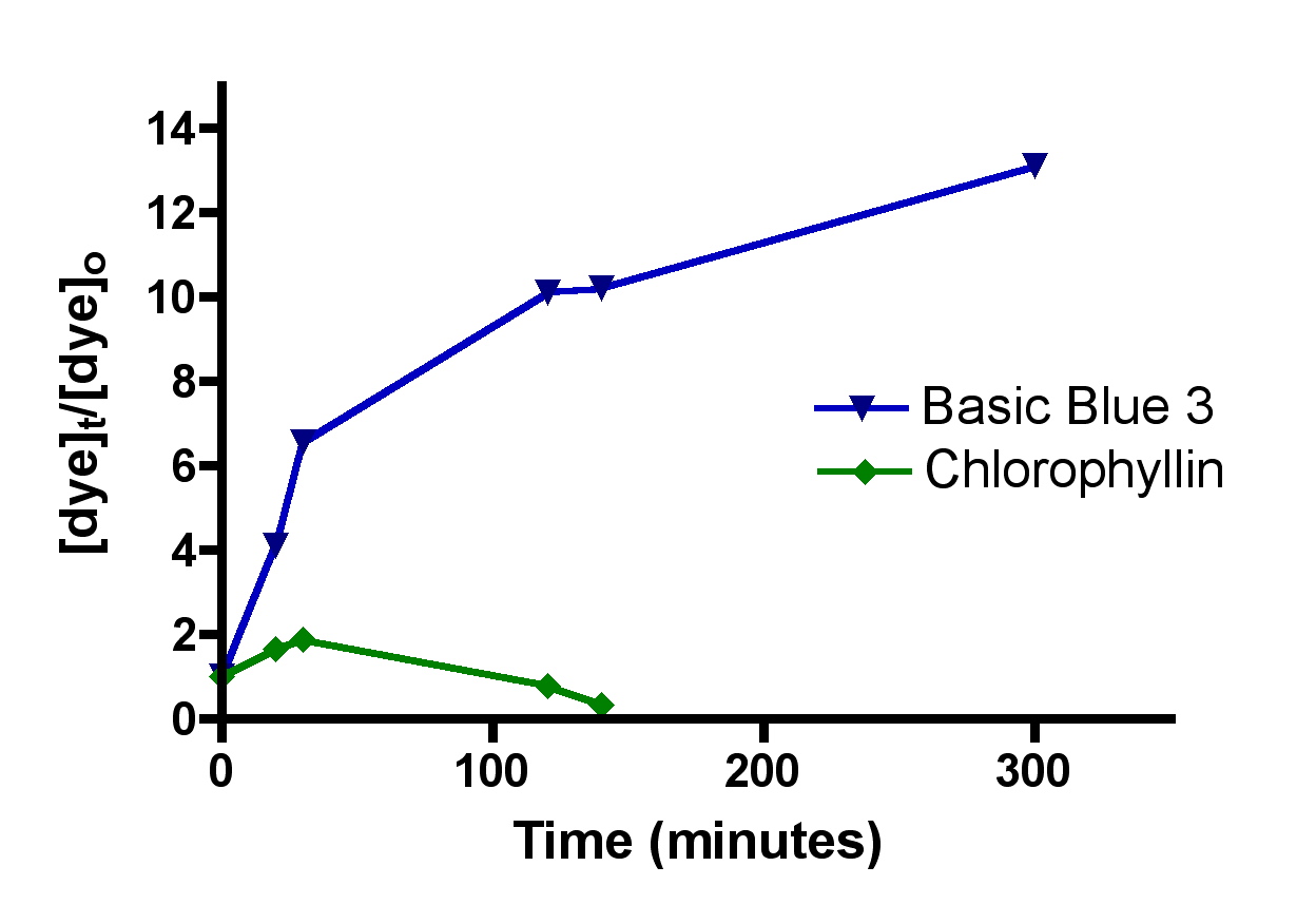
Figure 8. Leaching of both Basic Blue 3 and Chlorophyllin from Hydrocarbon2 infused with the dyes.
These leaching results do not negate the assumption underlying the kinetic analysis described in the Mathematical Modeling section, as long as the rate of removal data were recorded under an experimental protocol were the Hydrocarbon2 was not saturated. Given that the experiments were conducted under a regime where a large excess of HC2 binding sites compared with dye were evident (at least for ≥ 75 gms of HC2), it does not appear that saturation of the HC2 samples was achieved, and hence dye leaching during the trials is not likely to compromise the data.
GAC Comparison: Hydrocarbon2 vs. Black Diamond
A brief comparison of two different GAC’s, Hydrocarbon2 from Two Little Fishes and Black Diamond from Marineland, was pursued. For these trials, a 50 gm charge of GAC was used, the flow was set at 49 gph, and all four dyes were examined. The choice of a 50 gram GAC charge was made prior to the discovery that GAC amounts below 75 gm led to suboptimal rate constants (cf. Table 2). Therefore, it is not appropriate to compare directly the rate constants reported in Table 4 below, which were derived from the 50 gm GAC charges, with the maximal values from Table 1 derived from the 75 – 200 gm Hydrocarbon2 charges. Nevertheless, the relative rate constants for the different dyes from these 50 gram GAC experiments should be directly comparable, and the conclusions drawn from these comparisons should be unaffected by the channeling problems posited earlier with the < 75 gm Hydrocarbon2 charges.
Figure 9 displays the change in concentration of the four dyes as time increases for both Black Diamond and Hydrocarbon2. As noted earlier, Basic Blue 3, Acid Yellow 76 and Fluorescein all behave similarly to each other, but chlorophyllin is adsorbed by Black Diamond no better than it is by Hydrocarbon2. However, there is a conspicuously steeper drop-off in dye concentration for the other three dyes with Black Diamond compared to Hydrocarbon2. This steeper drop-off is reflective of a larger rate constant for dye removal, and these differences can be quantified using Eq. (13), as shown in Table 4.
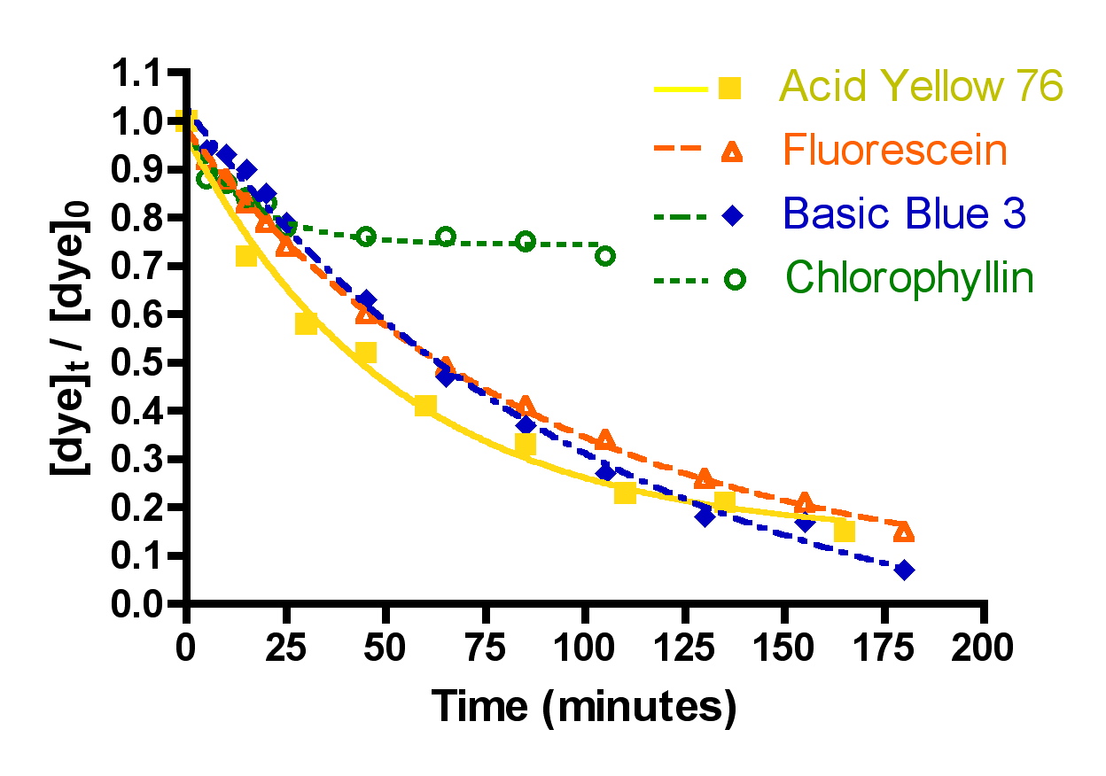
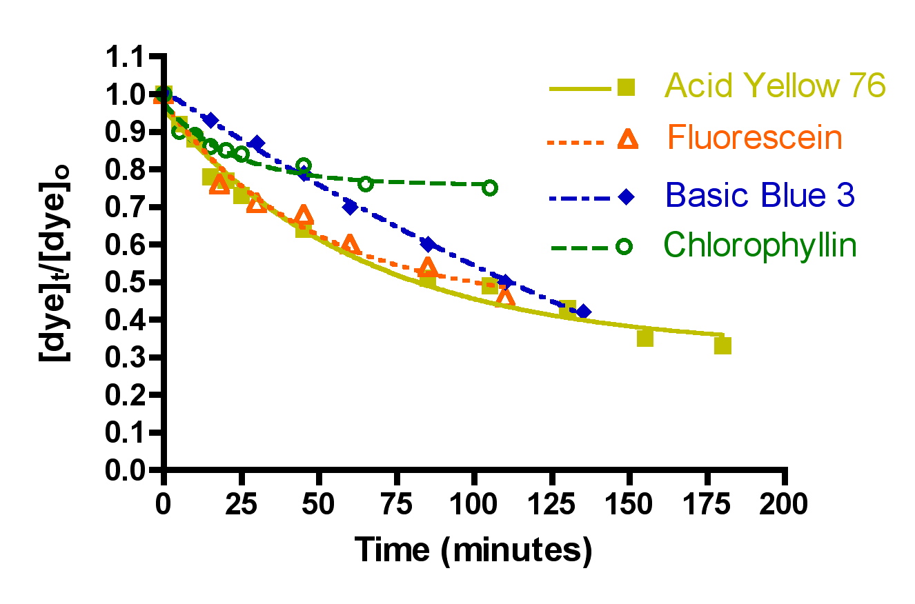
Figure 9. Dye removal by Black Diamond (top) and Hydrocarbon2 (bottom) at 49 gph flow, using 50 gm of GAC.
For the three dyes that do seem to be susceptible to significant adsorption by GAC (Acid Yellow 76, and Fluorescein/Basic Blue 3 combined), the rate constants k for dye removal are approximately twice as large with Black Diamond as they are with Hydrocarbon2. Correspondingly, the derived t90 values with Black Diamond are about half of those with Hydrocarbon2. These data lead to the clear conclusion that Black Diamond removes these dyes more rapidly than Hydrocarbon2, and by inference, DOC in general. Whether the factor-of-two difference with the dyes translates to a similar ratio with authentic DOC removal in a marine tank is unknown, but it seems likely that the large advantage enjoyed by Black Diamond for dye removal will lead to enhanced rates of organic clearance for the aquarist.
| dye | GAC | ||
|---|---|---|---|
| HC2 | Black Diamond | ||
| Basic Blue 3 andFluorescein | k (L/mol-min) | 13 ± 0.7 | 28 ± 1 |
| r2 | 0.99 | 0.99 | |
| t90 (hours) | 7.1 | 3.3 | |
| Acid Yellow 76 | k (L/mol-min) | 11.9 ± 0.7 | 23 ± 1 |
| r2 | 0.97 | 0.98 | |
| t90 (hours) | 7.3 | 3.8 | |
| Chlorophyllin | k (L/mol-min) | 3.7 ± 0.4 | 3.9 ± 0.7 |
| r2 | 0.79 | 0.83 | |
| t90 (hours) | 23 | 21.6 | |
Aquarium Applications
How much GAC should I Use?
The answer to this question really depends on what the goal is. There are arguments for removing impurities rapidly (clearing a toxic substance) and for removing them slowly (don’t shock the corals with more light penetration), and so no one best GAC amount will fit all circumstances. Nevertheless, the data presented below (Figure 10) might be useful in establishing guidelines for selecting the appropriate amount of GAC for a given situation. These graphs illustrate the calculated time (in hours) required to cut the amount of DOC by 90% as a function of the mass of HC2 used, the tank water volume, and the amount of DOC assumed to be initially present.
What is the justification for the assumption that certain amounts of DOC are present? More succinctly, “Just how much DOC is in reef tank water?” Due to a lack of adequate assay methods at present, this quantity, while crucial to any DOC removal technology, can only be approximated. A reef tank has a certain amount of DOC present as a consequence of a balance between DOC production and DOC removal (by any method), but how can that amount be quantified?
Commercially available DOC measurement kits are uniformly disappointing in that they only detect a small class of organic substances. As part of an ongoing study of protein skimmer efficiency in removing proteins and other DOC from aquarium tank water, we are exploring an oxidation-based assay procedure for DOC quantification that utilizes commercially available protein measurement kits. Although it is beyond the scope of this article to elaborate on this procedure (see coming attractions: “Quantitative Evaluation of Protein Skimmer Performance”), our preliminary assays of both skimmed-and-GAC-treated and unskimmed/no-GAC marine tank water reveal DOC levels on the order of 0.5 – 1 ppm for GAC/skimmed tanks and 5-10 ppm for no-GAC/unskimmed tanks. Specifically, oxidizable organic levels from three skimmed and GAC-treated reef tanks and one fish-only tank are: 0.40 ppm, 0.42 ppm, 1.3 ppm, and 1.3 ppm. Similarly the oxidizable organic levels in two unskimmed/no-GAC reef tanks (soft corals, invertebrates and a few fish) are: 4.5 and 8.5 ppm. Since our assay only detects oxidizable organics, it is likely to underestimate the actual amount of DOCs, but probably not by a great amount. That is, the oxidizing agent employed in the assay is powerful enough to oxidize (and hence detect) molecules from many of the compound classes illustrated in Figure 1. We plan to employ this assay with specific members of these molecular classes to test this assumption, but those studies remain for the future. This admittedly small sample size will be taken as representative for the purpose of the calculations below. To incorporate these oxidizable organic concentration values in the calculations, we will use as arbitrary starting points the values of 1.0 ppm of DOC and 7.5 ppm of DOC to represent “cleaner” and “dirtier” tanks, respectively. It will be of some interest to obtain samples of aquarium water out of a wide range of tanks from the greater reefkeeping community to expand upon this data set and see if consensus values emerge for oxidizable organics that correlate to different husbandry techniques, or to determine if the oxidizable organic level varies significantly, for example, when the lights are on or off, or during the period after a tank feeding. Those studies are in the future. Of course, continual replenishment of DOC’s by active biological processes (at an unknown rate) would ensure that DOC removal would never be complete! However, it is only necessary to remove DOC at a rate commensurate with, or faster than, the rate of DOC production in order to bring the DOC levels down to some arbitrarily low value.
The same mathematical approach discussed in Section 1.4 can be used to address the more interesting question for aquarists: how long will it take to remove, say, 90% of the DOC from the initial starting point of either 1 ppm or 7.5 ppm? In this case, Eq. (14) is used, but with new values for the water volume and the initial concentration of the DOC (equivalent to 1 and 7.5 ppm, respectively, of an average 400 molecular weight compound). The values of m and k are those extracted from the BB3/Fluorescein removal experiments – hence, the value of the dye system as a model for DOC removal in an aquarium. An average xm value of 53 mg of DOC/gm of GAC is used, which is based solely on the BB3/Fluorescein Langmuir isotherm experiments. It is possible, even likely, that other dyes (or more generally, other organic structures that are components of DOC) have different saturation values. The measurement of a larger collection of xm values corresponding to a range of plausibly DOC-like molecules will have to await further experimentation. Nevertheless, we have correlated k and xm values only for the BB3/Fluorescein dyes, and so we will confine our further analysis to these inputs. The results are displayed in Figure 10, with the 1 ppm DOC data on the left, and the 7.5 ppm DOC data on the right.
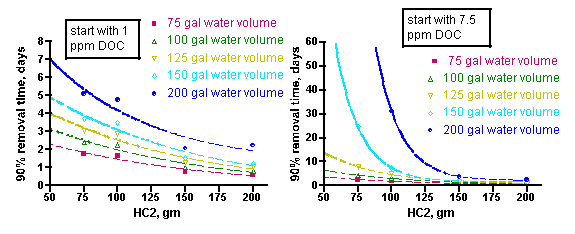
Figure 10. Calculated time for removal of 90% of DOC at starting points of 1 ppm DOC (left) and 7.5 ppm (right), as a function of tank water volume and amount of HC2 used.
The curves in these graphs can be fitted to the expressions shown in Eqs. (18 – 27) below, where t90 is the time, in days, required to deplete the DOC level to 10% of its original value, for a given amount of HC2 (indicated by “gm”). These mathematical relationships are strictly empirical and should not be extrapolated beyond the HC2 data range. Note that in the 7.5 ppm DOC case, the 200 gallon water volume contains too much DOC to be 90% absorbed by amounts of HC2 less than ~ 100g.
(18) (1 ppm DOC, 75 gallon) t90 = 3.7e(-0.008•(gm)) – 0.2, r2 = 0.92
(19) (1 ppm DOC, 100 gallon) t90 = 5.1e(-0.0081•(gm)) -0.3, r2 = 0.93
(20) (1 ppm DOC, 125 gallon) t90 = 6.5e(-0.0084•(gm)) – 0.3, r2 = 0.93
(21) (1 ppm DOC, 150 gallon) t90 = 8.0e(-0.0084•(gm)) – 0.4, r2 = 0.93
(22) (1 ppm DOC, 200 gallon) t90 = 11.4e(-0.013•(gm)) + 1.2, r2 = 0.89
(23) (7.5 ppm DOC, 75 gallon) t90 = 6.7e(-0.012•(gm)) + 0.04, r2 = 0.96
(24) (7.5 ppm, 100 gallon) t90 = 14e(-0.016•(gm)) + 0.3, r2 = 0.98
(25) (7.5 ppm DOC, 125 gallon) t90 = 41.2e(-0.023•(gm)) + 0.74, r2 = 0.99
(26) (7.5 ppm DOC, 150 gallon) t90 = 1441e(-0.055•(gm)) + 1.8, R2 = 0.99
(27) (7.5 ppm DOC, 200 gallon) t90 = 8001e(-0.056•(gm)) + 2.3, r2 = 0.99
How might an aquarist use this information to answer the question “How much GAC should I use?” The aquarist will have to estimate the water volume of the system (for an accurate and simple way to calculate system water volumes, see http://www.reefkeeping.com/issues/2006-04/pr/index.php, Experiment 3), and then make a guess as to whether their tank has a low level of DOC’s (~ 1 ppm in a system with adequate nutrient removal) or a high level (~ 7.5 ppm in a system with poor/absent nutrient removal). For example, a system with 150 gallons of total water volume that is adequately skimmed (or subjected to other effective nutrient removal, assume [DOC] = 1 ppm) would be characterized by the aqua curve on the left-hand graph in Figure 10. By interpolating from that curve (or, more quantitatively, by using the expression of Eq. (21)), an aquarist can conclude that a 200 gram charge of HC2 should remove about 90% of the DOC in approximately 1.1 days, but a 75 gram portion of HC2 would take approximately 3.9 days to achieve the same result.
Of course, DOC is continually being introduced via feeding and metabolic processes, and so the ultimate question of how much GAC to use in order to deplete the DOC concentration to some arbitrarily low target value in the aquarium requires knowledge of the rate of DOC production and not just the rate of DOC removal. Since this former quantity is not measurable by any simple means, only half an answer is possible at this point in the analysis (however, see Section 3.2). Of course, using a larger charge of HC2 would be more likely to allow the aquarist to “keep ahead” of the DOC production rate.
When Should I Change My GAC?
The useful lifetime of a GAC charge will depend on a host of factors, including the amount of GAC employed, the tank water volume, and the steady-state level of DOCs present. For the purpose of these calculations, we define a quantity, t90, as the time when 90% of the GAC’s DOC absorption capacity has been utilized. Using the experimentally determined k values from Table 2, the 53 mg-of-dye/gm-of-HC2 saturation value derived from Table 1, and an arbitrary starting DOC concentration (either 1 ppm or 7.5 ppm as per the discussion in Section 3.1), the KinTekSim program can decipher the kinetics of Eq. (15) and calculate the concentrations of [DOC] and [GACbs] as a function of time, when both [PoOP] and k1 are user-defined inputs. One important test of any kinetics simulation approach for extracting useful information from complex systems is the ability to reproduce experimental data with fidelity. Towards this end, we examined the simulated removal of DOC from tank water with the DOC input mechanism turned off ([PoOP]•k1 set to 0). This test simulation is equivalent to the simple Eq. (1) case, and the calculated output of [DOC] as a function of time matched closely the experimental data shown in Figure 4, at least for the 3 cases examined: 50, 100, and 200 gms of HC2 in the 4 gallon volume of the experimental reservoir.
For the initial [DOC] = 1 ppm series, we examined [PoOP]•k1 values spanning the range of 0.1 ppm/day to 1 ppm/day for a 100 gallon water volume and a 100 gm HC2 charge (chosen to be in the middle of the water volume and GAC amount ranges), and recorded the calculated average DOC levels during the time t = 0 days to t = t90 days. The goal of this exercise was to iterate through the [PoOP]•k1 values until readings for [DOC]ave fell into the experimental range of ~ 0.5 – 1.0 ppm observed in actual marine tanks (see section 3.1).
The range of [PoOP]•k1 values that met this criterion centered around 0.2 ppm/day, and so for the range [PoOP]•k1 = 0.15 – 0.35 ppm/day, we expanded our calculations to include “extreme” values of tank water and GAC used, in the hopes of capturing the full spread of [DOC] amounts that might emerge from these simulations. These data are recorded in Table 5. A similar approach was employed for the dirtier tank, using [DOC] = 7.5 ppm as the starting point. These latter calculations required substantially greater DOC introduction to achieve the [DOC]ave » 4 – 8 ppm level, and the relevant [PoOP]•k1 values turned out to be an order-of-magnitude higher that in the cleaner tank case where the initial [DOC] = 1 ppm. Is this a realistic outcome? It is important to recognize that the aquarium water which measured ~ 4 – 8 ppm of oxidizable organics with our protein assay was taken from unskimmed tanks, whereas the water that measured 0.5 – 1 ppm of oxidizable organics was taken from skimmed tanks. Our simulations do not account for any other methods of nutrient removal besides GAC, so skimming or water changes are not recognized. Therefore, in order to elevate [DOC]ave to the ~ 4 – 8 ppm level characteristic of the unskimmed (“dirty”) tanks for these simulations, we cannot remove less DOC (as implied by the absence of skimming) and so we must increase the rate of DOC introduction (larger [PoOP]•k1).
Since all of the calculated [DOC]ave values in Table 5 fall within the experimental ranges of measured tank oxidizable organic levels, which values do we choose to continue on with the simulations? Since the tank water assay detects only oxidizable organics, it seemed prudent to choose a higher end value to account for the undetected non-oxidizable components of DOC. For this reason, we selected [PoOP]•k1 = 0.30 ppm/day at 1 ppm of starting DOC as the input rate of DOC production for the remaining simulations, and [PoOP]•k1 = 3.0 ppm/day for the simulations starting with 7.5 ppm of DOC. Once a [PoOP]•k1 value is chosen, it must be used for all of the other tank-volume/GAC-amount variations examined in the respective 1 ppm or 7.5 ppm DOC series, as [PoOP]•k1 will not scale with either water volume or GAC mass. This constraint leads to some spread in the data, as not every volume/GAC pairing will be best described by [PoOP]•k1 = 0.30 ppm/day.
| Starting [DOC] = 1.0 ppm | Starting [DOC] = 7.5 ppm | ||||
|---|---|---|---|---|---|
| [PoOP]•k1ppm/day | [DOC]ave ppm | [DOC] at t90 ppm | [PoOP]•k1ppm/day | [DOC]ave ppm | [DOC] at t90, ppm |
| 0.15 | 0.57 | 1.2 | 1.0 | 3.7 | 4.5 |
| 0.20 | 0.65 | 1.3 | 2.0 | 5.1 | 6.8 |
| 0.25 | 0.75 | 1.5 | 3.0 | 6.6 | 8.5 |
| 0.30 | 0.87 | 1.7 | 4.0 | 7.1 | 10.1 |
| 0.35 | 0.98 | 2.0 | 5.0 | 7.9 | 11.7 |
The influence of the specific [PoOP]•k1 value on the desired calculated quantity, t90, can be seen from inspection of the data in Figure 11. These graphs depict the calculated DOC and GACbs concentrations as a function of time for a 100gallon/100 gm HC2 simulation, at different [PoOP]•k1 values (upper: 1 ppm starting DOC. lower: 7.5 ppm starting DOC). The intersections of the GACbs lines with the t90 lines indicate the time required to saturate 90% of the HC2 with DOC. Quantitatively, for the 1 ppm starting DOC series (upper graph): for [PoOP]•k1 = 0.25 ppm/day, t90 = 49 days; for [PoOP]•k1 = 0.30 ppm/day, t90 = 41 days, and for [PoOP]•k1 = 0.35 ppm/day, t90 = 36 days. So, if we guessed wrong for the [PoOP]•k1 value by 17%, we introduce a spread of about 14% into the final t90 values. That is, a spread in [DOC]ave of 0.75 – 0.98 ppm (from Table 5) correlates to t90 values of 36 – 49 days, or for the 100gallon/100gm case, the GAC will be 90% saturated at around 41 ± 6 days. Similarly, for the 7.5 ppm starting DOC series (lower graph), the following t90 values can be gleaned: for [PoOP]•k1 = 2.0 ppm/day, t90 = 5.0 days; for [PoOP]•k1 = 3.0 ppm/day, t90 = 3.9 days, and for [PoOP]•k1 = 4.0 ppm/day, t90 = 3.3 days. Once again, estimating [PoOP]•k1 incorrectly by 33% leads to an 18 – 28% error in the calculated t90 values. These potential errors carry much less significance in the starting [DOC] = 7.5 ppm case compared with the starting [DOC] = 1 ppm series, since the t90 values are so short. Basically, the HC2 saturates in just a few days, and it will likely matter little to the aquarist working under these conditions whether the exact saturation time is 3 days or 5 days. Given all of the assumptions that undergird this simulation, a conservative approach to interpreting these output values would seem prudent, and would require these rather large error bars. This lack of precision may be disquieting, but it is important to emphasize that the simulation results are clearly not consistent with, for example, a scenario where t90 values of 10 days or 100 days are calculated ([DOC] = 1 ppm case). This spread in the data is typical of kinetics simulations where the input parameters are uncertain. As a last point, note how the DOC concentration begins to rise significantly when the GAC is 90% saturated – this behavior is entirely consistent with the physical reality of the tank getting dirtier via DOC production when the DOC removal mechanism shuts down.
An interesting observation to emerge from these simulations is that, at least for the 100 gallon water volume/100 gm of HC2 case described by Table 5 and Figure 11, the GAC saturation times vary tremendously depending upon the clean/dirty state of the tank water. Under conditions of aggressive DOC removal (skimming, water changes, GAC use), the GAC charge should last over a month, but under more passive nutrient removal husbandry (no skimming? no frequent water changes?), the GAC charge will be depleted in just a few days.
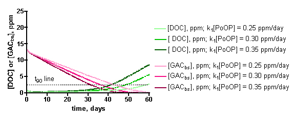
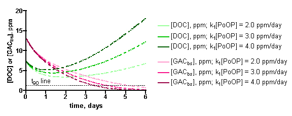
Figure 11. Examples of the KinTekSim output for a 100 gallon/100gm of HC2 simulation, using different values of the input parameter [PoOP]•k1. Upper graph: 1.0 ppm DOC starting point. Lower graph: 7.5 ppm starting point.
Extension of these simulations to a range of tank water volumes and GAC amounts will provide the aquarist with suggestions for GAC depletion times over a range of realistic usage scenarios. Using the [PoOP]•k1 values of 0.3/ day and 3.0/day for the 1 ppm and 7.5 ppm of [DOC] cases, respectively, simulations covering tank volumes of 75 – 200 gallons and HC2 amounts of 50 – 200 gm leads to the family of linear relationships that are shown in Figure 12 (starting [DOC] = 1 ppm on the left side, and starting [DOC] = 7.5 ppm on the right side). Each line represents a different tank water volume, and expresses the relationship between the amount of HC2 used (X-axis) and the corresponding time-of-use until the HC2 is 90% saturated (Y-axis). These relationships can be expressed by the mathematical formulae Eq. (28) – Eq. (37) below. In principle, all of these lines should pass through the origin of the graph (t90 = 0 when there is no HC2 present). However, the best-fit lines have small and positive Y-axis intercepts. This deviation from ideality is again a reminder of the role that assumptions and experimental error plays in any laboratory enterprise. Fortunately, for this case, the non-zero Y-intercepts only amount to < 10% of the final t90 readings. These mathematical relationships are strictly empirical and should not be extrapolated beyond the HC2 data range.
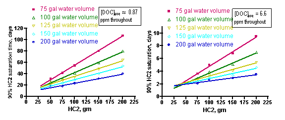
Figure 12. Calculated time to saturate 90% of the available HC2 binding sites as a function of amount of HC2, tank water volume, and starting DOC concentration (1 ppm (left) and 7.5 ppm (right)).
(28) (1 ppm DOC, 75 gallon) t90 = 0.51•(gm) + 3.7, r2 = 0.99
(29) (1 ppm DOC, 100 gallon) t90 = 0.37•(gm) + 5.2, r2 = 0.99
(30) (1 ppm DOC, 125 gallon) t90 = 0.27•(gm) + 8.3, r2 = 0.99
(31) (1 ppm DOC, 150 gallon) t90 = 0.23•(gm) + 6.2, r2 = 0.99
(32) (1 ppm DOC, 200 gallon) t90 = 0.16•(gm) + 7.6, r2 = 0.97
(33) (7.5 ppm DOC, 75 gallon) t90 = 0.046•(gm) + 0.22, r2 = 0.99
(34) (7.5 ppm, 100 gallon) t90 = 0.032•(gm) + 0.57, r2 = 0.99
(35) (7.5 ppm DOC, 125 gallon) t90 = 0.021•(gm) + 1.2, r2 = 0.98
(36) (7.5 ppm DOC, 150 gallon) t90 = 0.016•(gm) + 1.3, R2 = 0.94
(37) (7.5 ppm DOC, 200 gallon) t90 = 0.010•(gm) + 2.6, r2 = 0.93
How might an aquarist use this information to answer the question “When should I change my GAC?” Much as with the “How much GAC?” question addressed in Section 3.1, the aquarist will have to estimate the water volume of the system, and then make a guess as to whether their tank has a low level of DOC’s (~ 1 ppm in a system with adequate nutrient removal) or a high level (~ 7.5 ppm in a system with poor/absent nutrient removal). For example, a system with 150 gallons of total water volume that is adequately skimmed (or subjected to other effective nutrient removal, [DOC] ≤ 1 ppm) would be characterized by the aqua line on the left-hand graph in Figure 12. By interpolating from that line (or, more quantitatively, by using the expression of Eq. (31)), an aquarist can conclude that a 100 gram charge of HC2, for example, should be replaced in approximately 29 days, whereas a 200 gram portion of HC2 would last approximately 52 days before it became saturated with DOC’s. In a similar manner, an aquarist running an unskimmed (i.e., [DOC] at approximately 7.5 ppm) 75 gallon tank could use the magenta line in the right-hand graph of Figure 12 (or Eq. (33)) to estimate that a 100 gm HC2 charge will become saturated with DOC’s in approximately 4.8 days, and a 200 gm portion of HC2 would last about 9 days. Clearly, very nutrient rich tanks will require better means of DOC export than only GAC-based removal!
Conclusions
Aquarists who choose to use granular activated carbon (GAC) to aid in water purification are faced with two over-arching questions: “How much GAC should I use?”, and “When should I replace my GAC?”. Through a combination of experimentation using dyes as surrogates for dissolved organic carbon (DOC) and computer simulations of the DOC introduction/removal process, we can suggest tentative answers to these questions (Figures 10 and 12). The answers depend on three aquarist input quantities: the amount of DOC present, the amount of GAC used, and the tank water volume. The latter two metrics are easy to come by, but quantifying the amount of DOC present must still await reliable assay kits. Nevertheless, data from a small sampling of tanks provides guidance on this point, as both low-nutrient (~ 0.5 – 1 ppm of measurable oxidizable organics) and high-nutrient (~ 4 – 8 ppm of measurable oxidizable organics) water samples seem to correlate with either the presence or absence of an efficient protein skimmer. Certainly, a broader survey of marine tanks in the future will help refine these numbers.
In the final analysis, this study presents results that are based on model systems and not real operational marine tanks. We have made a case for the extrapolation of these model system conclusions to marine aquariums, but ultimately each aquarist will have to find their own comfort level regarding the validity of this connection.
Acknowledgment
We thank the Pennsylvania State University, the PSU Center for Environmental Kinetics Analysis (National Science Foundation grant # CHE-0431328) and du Pont de Nemours and Company for their financial support of this work.
References
- Alberts, B.; Johnson, A.; Lewis, J.; Raff, M.; Roberts, K.; Walter, P. 2002. Molecular Biology of the Cell, 4th Ed. Garland Science, Taylor and Francis Group, Boca Raton, Florida.
- Bansal, R. C.; Goyal, M. 2005. Activated Carbon Adsorption. Taylor and Francis Group, Boca Raton, Florida.
- Baup, S.; Jaffre, C.; Wolbert, D.; LaPlanche, A. 2000. “Adsorption of Pesticides onto Granular Activated Carbon: Determination of Surface Diffusivities Using Simple batch Experiments.” Adsorption, 6, 219-228.
- Bingman, C. A. 1996. “Aquatic Humic Acids.” Aquarium Frontiers, 3, 11-14.
- Callot, H. J.; Ocampo, R. 2000. Porphyrin Handbook. Kadish, K. M.; Smith, K. M.; Guilard, R., Eds., Academic Press, San Diego, California, 349-398.
- Cerreta. 2006. “Experiment: Is All Granular Activated Carbon (GAC) Created Equally?” Reef Central Chemistry Forum.
- Cheremisinoff, N. P.; Cheremisinoff, P. N. 1993. Carbon Adsorption for Pollution Control. PTR Prentice Hall, Englewood Cliffs, New Jersey.
- Chien, J.-Y. 1948. “Kinetic Analysis of Irreversible Consecutive Reactions.” J. Am. Chem. Soc., 70, 2256-2261.
- Francois, R. 1990. “Marine Sedimentary Humic Substances: Structure, Genesis, and Properties.” Rev. Aquatic Sci., 3, 41-80.
- Ganguly, S. K.; Goswami, A. N. 1996. “Surface Diffusion Kinetics in the Adsorption of Acetic Acid on Activated Carbon.” Separations Sci. Tech., 31, 1267-1278.
- Gillam, A. H.; Wilson, M. A. 1986. “Structural Analysis of Aquatic Humic Substances by NMR Spectroscopy.” ACS Symposium Series: Organic Marine Geochemistry, 305, 128-141.
- Harker, R. 1998. “Granular Activated Carbon in the Reef Tank: Fact, Folklore and Its Effectiveness in Removing Gelbstoff -Parts 1 and 2.” Aquarium Frontiers, May and June issues. http://www.reefs.org/library/aquarium_frontiers/index.html.
- Harvey, G. R.; Boran, D. A.; Chesal, L. A.; Tokar, J. M. 1983. “The Structure of Marine Fulvic and Humic Acids.” Marine Chem. 12, 119-132. For a commentary on the conclusions drawn in this article, and a rebuttal, see: Laane, R. W. P. M. 1984. “Comment on the Structure of Marine Fulvic and Humic Acids.” Marine. Chem. 15, 85-87, and Harvey, G. R. Reply: Comment on the Structure of marine Fulvic and Humic Acid.” Marine Chem. 15, 89-90.
- Homes-Farley, R. 2004 “Organic Compounds in the Reef Aquarium.” Reefkeeping, 10, http://www.reefkeeping.com/issues/2004-10/rhf/index.php.
- Hovanec, T. 1993. “All About Activated Carbon.” Aquarium Fish Magazine, 5, 54-63.
- Khan, A. R.; Ataullah, R.; Al-Haddad, A. 1997. “Equilibrium Adsorption Studies of Some Aromatic Pollutants from Dilute Aqueous Solutions on Activated Carbon at Different Temperatures.” J. Colloid Interface Sci. 194, 154-165.
- Lliopoulos, A.; Reclos, J. G.; Reclos, G. J. 2002. “Activated Carbon.” Fresh Water and Marine Aquarium, January issue.
- Kvech, S.; Tull, E. 1997. “Activated Carbon.” Water Treatment Primer, Civil Engineering Department, Virginia Tech, http://ewr.cee.vt.edu/environmental/teach/wtprimer/carbon/sketcarb.html.
- Noll, K. E.; Gouranis, V.; Hou, W. S. 1992. Adsorption Technology for Air and Water Pollution Control. Lewis Publishers, Chelsea, Michigan.
- Rashid, M. A. 1985. Geochemistry of Marine Humic Compounds. Springer-Verlag, New York, New York.
- Romankevich, E. A. 1984. Geochemistry of Organic Matter in the Ocean. Springer-Verlag, New York, New York.
- Sardessal, S.; Wahidullah, S. 1998. “Structural Characteristics of Marine Sedimentary Humic Acids by CP/MAS 13C NMR Spectroscopy.” Oceanologica Acta, 21, 543-550.
- Schiemer, G. 1997. “About Activated Carbon.” Aquarium Frontiers, July issue.
- Singh, S.; Yenkie, M. K. N. 2006. “Scavenging of Priority Organic Pollutants from Aqueous Waste Using Granular Activated Carbon.” J. Chinese Chem. Soc. 2006, 53, 325-334.
- Spartan’04. Wavefunction, Inc. Irvine, CA.
- Suzuki, M. 2001. “Activated Carbon Adsorption for Treatment of Agrochemicals in Water.” Environmental Monitoring and Governance in the East Asian Hydrosphere Symposium Abstracts, http://landbase.hq.unu.edu/Symposia/2001Symposium/abstracts/06Suzuki.htm.
- Walker, G. M.; Weatherley, L. R. 2000. “Prediction of Bisolute Dye Adsorption Isotherms on Activated Carbon.” Trans. Institut. Chem. Eng., 78, 219-223.
- Walker, G. M.; Weatherly, L. R. 1999. “Kinetics of Acid Dye Adsorption on GAC.” Water Res. 33, 1895-1899.
0 Comments