

Last month we discussed the various components of the carbonate system in sea water. We identified each parameter, mentioned typical values for these parameters in natural sea water, and discussed briefly why these parameters are important for aquarists to consider. This month we will begin to tackle how each of these components interacts with the others. Simply put, this article will examine how the carbonate system works.
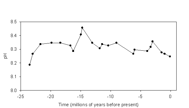
Figure 1. Mean surface ocean pH over the last 23.5 million years. After Pearson and Palmer, 2000.
The Control of Seawater pH
The pH of typical surface sea water averages about 8.20 today, was nearer 8.30 during the preindustrial period, and was closer to 8.45 during the last glacial maximum (~20,000 years ago). These values are typical for oceanic pH over at least the last 23.5 million years. Indeed, mean oceanic pH has varied only within the range of about 8.2-8.45 during this period (Figure 1). One might ask why the pH of the shallow ocean has tended to stay within this range, even over comparatively long periods of time? Why isn’t the pH of the ocean 6? Why not 10? The answer brings us to one of the most important interactions in the carbonate system.
Carbon dioxide gas is present in the atmosphere and dissolves into sea water according to its partial pressure, as described by Henry’s Law:
[CO2*] = KH × pCO2
where [CO2*] is the concentration of dissolved CO2 in the water, KH is a Henry’s Law constant for CO2 in sea water (at a given temperature and pressure) and pCO2 is the partial pressure of CO2 in the atmosphere. The surface ocean will tend to take up a particular amount of CO2 and that amount is directly proportional to the concentration of CO2 in the air overlying that water. The exchange of CO2 between the surface ocean and the atmosphere is constantly ongoing. That is, individual molecules of CO2 are always moving from the surface ocean to the atmosphere and from the atmosphere to the surface ocean. These two pools exchange CO2 back and forth all the time. If the ocean-atmosphere system is near equilibrium then the rate of exchange of CO2 will be equivalent in both directions, ocean to atmosphere and atmosphere to ocean, ensuring no net change in the size of either pool.
This exchange can fall out of equilibrium if either the atmospheric or oceanic pool of dissolved CO2 is altered. For example, if there is a net release of CO2 into the atmosphere, increasing the atmospheric concentration, the surface ocean will become undersaturated with respect to CO2 given the new, higher atmospheric concentration. More CO2 will dissolve from the atmosphere into the ocean than from the ocean to the atmosphere. The imbalanced exchange increases the amount of dissolved CO2 in the ocean until the atmospheric and oceanic pools eventually reach a new equilibrium. In this case the amount of CO2 dissolved in the surface ocean and in the atmosphere will both be higher at the new equilibrium than they were previously. Conversely, if there is a net removal of CO2 from the atmosphere the reverse process will play out. The ocean will lose CO2 to the atmosphere until the two reach a new equilibrium. In this case the amount of CO2 dissolved in the surface ocean and in the atmosphere will both be lower than they were previously.
When CO2(g) dissolves into water it reacts with that water to produce carbonic acid (H2CO3). Adding an acid to sea water (or any solution), all else equal, reduces the pH. The release of CO2 into the atmosphere results in an increase in the concentration of atmospheric CO2, an increase in the amount of dissolved CO2 in the surface ocean, an increase of the amount of carbonic acid, and a reduction of oceanic pH. The removal of atmospheric CO2 results in a reduction in the concentration of atmospheric CO2, a reduction of the amount of CO2 dissolved in the surface ocean, a reduction of the amount of carbonic acid, and an increase in oceanic pH. In today’s atmosphere the partial pressure of CO2 is about 387 μatm and is very quickly increasing due to the burning of fossil fuels. We’ll discuss how ocean chemistry is changing as a result of fossil fuel burning in a future article. In pure water the dissolution of CO2 from today’s atmosphere produces a mildly acidic solution with pH = 5.6 — much lower than the pH of sea water. Clearly there must be a component besides dissolved CO2 that affects seawater pH.
Total alkalinity is that other component. While CO2(g) produces an acid when dissolved in water, certain minerals also dissolve into sea water and produce bases. The most important compounds that provide alkalinity in the ocean are the carbonates (CaCO3, MgCO3, etc.) and the silicates (Mg2SiO4, KAlSi3O8, etc.). When carbonates dissolve they release HCO3– and CO32- ions into solution, providing alkalinity. Silicates tend to react with carbonic acid, derived from atmospheric CO2, and likewise release HCO3– and CO32- ions into solution. Borates also contribute a small portion of the total alkalinity (~2.9%) while other sources (e.g., phosphates) account for a very small portion (negligible for our purposes). Thus we have a dynamic system that controls seawater pH: CO2(g) in the atmosphere dissolves
into sea water, produces an acid, and pushes the pH lower. Certain minerals dissolve in the ocean (or on land and are transported to the ocean in runoff), contribute to the total alkalinity, and push the pH higher. Sea water is buffered by opposing forces of dissolved CO2 and total alkalinity (Figure 2). If the alkalinity in sea water were completely removed but atmospheric CO2 remained unchanged the pH would fall to about 5.46 (at equilibrium with the atmosphere) due to the dissolution of CO2. Alternatively, if the total CO2 (TCO2) were stripped from sea water but alkalinity remained unchanged the pH would rise to 10.6. It is the interplay between these two parameters that produces the pH we measure.
Over long time scales a variety of biological and geochemical processes work together to determine the amount of CO2 dissolved in the atmosphere and the ocean as well as the total alkalinity of oceanic water. Feedbacks among these various mechanisms have kept long-term oceanic pH within about the range of 8.2-8.45 for at least the last 23.5 million years. Over short time scales, however, the pH of sea water can and does vary because of short-term variation in the amount of dissolved CO2 or the total alkalinity.
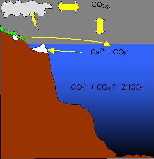
Figure 2. Carbon dioxide is exchanged between the atmosphere and the shallow ocean. Carbonates and other minerals dissolve into sea water, or are transported there in runoff, providing alkalinity. The interaction between dissolved CO2 and alkalinity largely determine seawater pH at any given moment.
The take-home message here is this: higher dissolved CO2 yields lower pH whereas lower dissolved CO2 yields higher pH, all else equal. pH and dissolved CO2 are inversely related. Conversely, higher alkalinity yields higher pH while lower alkalinity yields lower pH, all else equal. pH and alkalinity are directly related.
More often than not the supplementation schemes that we use to control alkalinity in captivity (whether a buffer, two-part system, calcium reactor, etc.) affect both alkalinity and dissolved CO2 at the same time. Hence the question of how a supplement or supplementation system affects tank pH becomes a more complex problem. We will consider these more complex interactions next month. For now let us consider just the basic relationship among dissolved CO2, alkalinity, and pH mentioned above. Reducing dissolved CO2 or increasing alkalinity raises pH. Increasing dissolved CO2 or reducing alkalinity lowers pH.
The other parameters of the carbonate system, calcium and magnesium, do not directly affect seawater pH. Instead, it is the interaction between total CO2 and total alkalinity that is responsible for determining the pH in our tanks, and in the ocean. In nature total alkalinity is nearly conservative in its behavior (i.e., varies simply due to altered salinity) over short timescales (< 100,000 yrs), thus it is primarily variation in dissolved CO2 (and hence atmospheric CO2) that determines oceanic pH. In our aquaria we have the opportunity to manipulate both dissolved CO2 and alkalinity to arrive at a desired pH.
The Concept of Saturation State
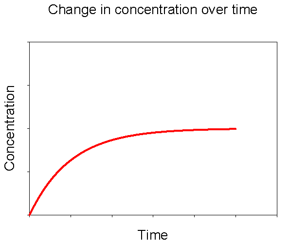
Figure 3. Change in concentration of dissolved CaCO3 over time upon adding solid CaCO3 to a solution initially devoid of dissolved CaCO3.
Let’s imagine a simple experiment. We fill a beaker with deionized water. Next we drop in a few pieces of solid calcium carbonate (CaCO3). What will happen? As you may have guessed, over time some of the CaCO3 will dissolve into the water. If we periodically measure the concentrations of dissolved calcium and carbonate, we’ll see a pattern like that in Figure 3. Initially there will be no dissolved CaCO3 in the water. When we add solid CaCO3 it dissolves quickly at first. As the concentration of dissolved CaCO3 increases over time the rate of net dissolution slows down. Eventually the concentration of dissolved CaCO3 plateaus. Note that this does not mean that there is no longer any dissolution taking place, but that the rate of dissolution and precipitation are equal, producing no net change in concentration thereafter.
Let’s now consider a similar experiment. To begin this experiment, instead of putting in solid CaCO3 we add a large amount of the dissolved components (e.g., a calcium chloride salt and a sodium carbonate salt). What will happen this time? This time we’ll see the reverse process: the precipitation of solid CaCO3 from the dissolved components. As seen in Figure 4, the concentrations begin at some high level and the rate of precipitation is fast. Over time the concentrations drop as does the rate of net precipitation. Eventually the concentration of dissolved CaCO3 plateaus, indicating that the rate of precipitation is equal to the rate of dissolution.
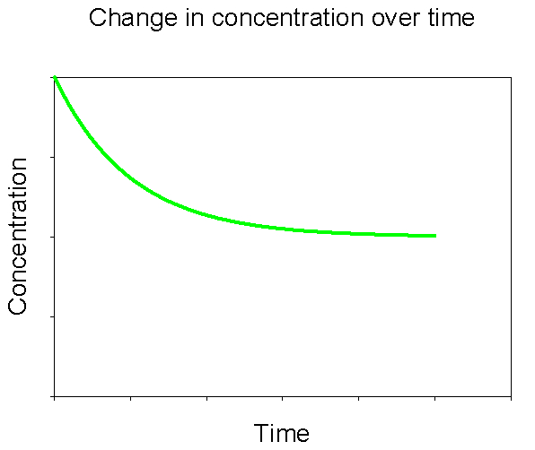
Figure 4. Change in concentration of dissolved CaCO3 over time after initially adding a large amount of dissolved CaCO3 to solution.
If we plot the data for both of these experiments on the same graph, we see that they converge to the same value for dissolved CaCO3 (Figure 5).
The value that these two curves converge to is the solubility of CaCO3 in deionized water, at a given temperature and pressure. We would see a similar pattern were we to conduct these experiments with any mineral. The parameters that would change for a different mineral would include the value that the curves converge to (= the solubility) and the amount of time required to reach that value. We can describe the solubility of CaCO3 using the following equation,
Ksp = (Ca2+)(CO32-)
where (Ca2+) and (CO32-) are the activities of calcium and carbonate ions, respectively, and Ksp is the solubility product of CaCO3. As we mentioned last month in our discussion of pH, ion activity is equivalent to ion concentration in solutions with very low ionic strength (= very little dissolved minerals). In a salty solution like sea water the activity of Ca2+ and CO32- will be much lower than the concentrations because of interactions with other ions. For convenience, the solubility product (Ksp) can be transformed for use in sea water. Calcium and carbonate ion activities are replaced with concentrations yielding an apparent solubility product (Ksp`):
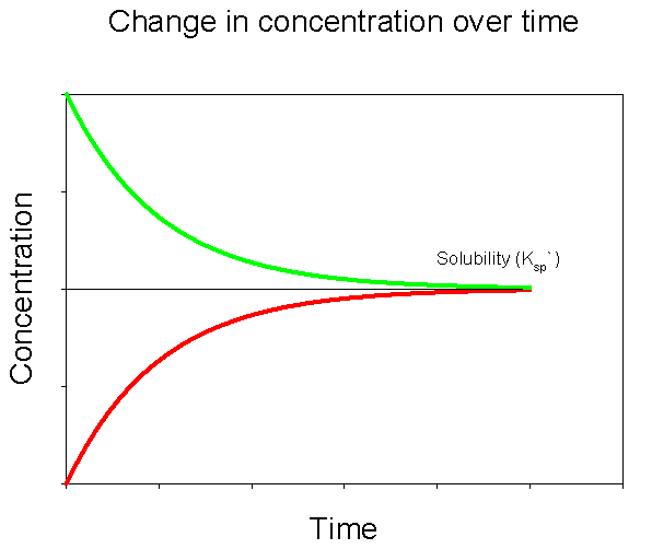
Figure 5. Change in concentration of dissolved CaCO3 over time upon adding solid CaCO3 to a solution initially devoid of dissolved CaCO3 (red) and after initially adding a large amount of dissolved CaCO3 to solution (green).
Ksp` = [Ca2+][CO32-]
Ksp` represents the value to which the curves above converged. At a given temperature and pressure it is simply a constant, a number that represents how much CaCO3 we would expect to dissolve. In the first experiment above, our solution was initially undersaturated with CaCO3 and took time to come up to saturation as CaCO3 dissolved. In the second experiment our solution was initially supersaturated and took time to come down to saturation as CaCO3 precipitated. We can express the degree of saturation (supersaturation, undersaturation, or saturation) by taking a ratio of the amount of CaCO3 actually dissolved in a water sample to the value that we would expect to be dissolved at equilibrium. This ratio is called the saturation state, and is given the symbol Ω:
Ω = [Ca2+][CO32-]/Ksp`
If Ω = 1 then our solution is exactly at saturation—there is the same amount of CaCO3 dissolved as we would expect to dissolve. We’d be at the point where the two curves above converge. If Ω < 1 then the solution is understurated and we would expect net dissolution, like in the first experiment. If Ω > 1 then the solution is supersaturated and we would expect net precipitation, like in the second experiment. The saturation state simply compares the amount of CaCO3 dissolved in the water to the amount that we expect should dissolve.
Rates of CaCO3 dissolution and precipitation are proportional to the saturation state (Mucci, 1983). That is, CaCO3 dissolves faster if the saturation state is really low than if the saturation state is just a little low, like in our first experiment above. Likewise, CaCO3 precipitates faster if the saturation state is really high instead of just a little high, like in our second experiment above.
Saturation state will change if any of the three parameters used to calculate it change:
- Ksp`
- Ca2+ concentration
- CO32- concentration.
Ksp`, representing the amount of CaCO3 we expect to dissolve, can be altered by changes in temperature or pressure. CaCO3 is more soluble at low temperatures and less soluble at high temperatures, unlike most solids. CaCO3 is also more soluble at very high pressure than at lower pressure. While the temperature effect can be important in aquaria in areas of local high temperature (e.g., on heaters, inside pumps) or over wide geographic areas in nature (e.g., tropics to polar regions), the day-to-day or seasonal variation in temperature typical on a coral reef or in an aquarium has only a modest impact on Ksp`. The effects of pressure are important in considering CaCO3 solubility in the shallow ocean compared to the deep sea, but not on coral reefs or in aquaria.
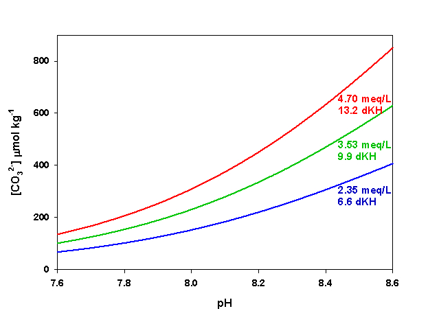
Figure 6. Effects of pH on CO32- concentration at three levels of alkalinity. Calculated using co2sys (Lewis and Wallace, 1998) assuming S = 35, T = 25 °C, P = 1 atm, and negligible total phosphate and silicate concentrations.
Calcium concentration is conservative in sea water (as discussed in Part I). Oceanic calcium concentration has in fact changed quite significantly over long timescales (millions of years), but over geologically short time scales (< 100,000 yrs) Ca2+ concentration does not and truly cannot change too much in the ocean. This is largely a result of the comparatively high background concentration of Ca2+ in the ocean. To significantly change the Ca2+ concentration of sea water requires the precipitation or dissolution of truly massive quantities of minerals. Even at maximal rates of dissolution or precipitation in nature, typically millions of years are required to substantially change the calcium concentration of sea water. Calcium concentration can, however, be manipulated over a wide range in aquaria.
The last parameter, CO32- concentration, is the one that is most likely to cause significant variation in Ω both in nature and in aquaria. Because of the nearly conservative behavior of alkalinity in the ocean, for a given salinity CO32- concentration varies primarily as a function of pH, and hence of dissolved CO2. In captivity we can manipulate both alkalinity and pH (via CO2), yielding a potentially very large range of values for CO32- concentration in aquaria. An increase in either alkalinity or pH will result in an increase in CO32- concentration. Conversely, a decrease in either alkalinity or pH will result in a decrease in CO32- concentration (Figure 6).
By manipulating Ca2+ concentration, total alkalinity, and pH we are able to arrive at a wide range of values for Ω in aquaria, but what sort of range? The answer depends heavily on the type of CaCO3 mineral under consideration.
Calcium Carbonate Mineralogy
The compound CaCO3 can form several different minerals. These different forms (referred to as polymorphs) have different physical arrangements of ions in the lattice structure of the crystals. While it may at first seem strange that the same ions can be used to form different minerals, elemental carbon (C) provides an example that may be more familiar. Pure carbon can assemble into several different crystalline structures. Among these different forms are graphite (i.e., what’s in pencils) and diamond. The spatial arrangement of carbon atoms in the crystal lattice of these two minerals is distinct. In graphite the carbon atoms make a series of sheets, like the pages of a book. It’s easy to separate those sheets, hence why graphite readily leaves smudges when rubbed against a surface. Diamond, unlike the sheets of carbon atoms in graphite, is a cubic crystal which gives diamond its strength. The different physical arrangement of carbon atoms gives graphite and diamond very different physical properties. Graphite is very soft while diamond is the hardest known mineral.
Similarly, CaCO3 can form crystals that have different arrangements of the two ions. The distinct arrangements give the minerals somewhat different physical properties. The three most common polymorphs of CaCO3 produced by calcifying organisms are low-magnesium calcite (low-Mg calcite), high-magnesium calcite (hi-Mg calcite) and aragonite. Both hi- and low-Mg calcite have a rhombohedral lattice structure, but Mg2+ replaces many of the Ca2+ in the lattice of hi-Mg calcite. Aragonite has an orthorhombic lattice. Other polymorphs such as vaterite occur in some organisms, but are relatively rare in the completed shells/skeletons.
One of the most important physical properties that changes among these polymorphs is the solubility. We defined the saturation state, Ω, as the ratio of the amount of CaCO3 dissolved in a water sample to the amount we expect to dissolve. Since the various CaCO3 polymorphs have different solubilities, we must us the Ksp` that is appropriate for the mineral we are interested in. Low-Mg calcite and aragonite are reasonably similar in their composition whether they are made by different organisms or precipitated abiotically. Therefore, their solubility has been well characterized in sea water over a range of conditions. Hi-Mg calcite is truly a mixed solid made of mostly CaCO3, but also a significant quantity of MgCO3. Calcite that is < 4 mol % MgCO3 is typically classified as low-Mg calcite whereas calcite that is > 4 mol % MgCO3 is classified as hi-Mg calcite. Usually hi-Mg calcite formed by marine organisms ranges from about 8-20 mol % MgCO3 while low-Mg calcite is not more than a few mol % MgCO3. Magnesium carbonate is much more soluble than CaCO3 in sea water. Hence, the more Mg2+ there is in the hi-Mg calcite, the more soluble it will be. The proportion of Mg2+ in hi-Mg calcite can be variable depending on the conditions in which it was formed and/or the organism that formed it, leading to differences in solubility. As a result, the Ksp` for hi-Mg calcite is not as well characterized as for low-Mg calcite or aragonite. Roughly speaking, however, hi-Mg calcite is about 1.5-1.7 times as soluble as aragonite in modern sea water while aragonite is about 1.5 times as soluble as low-Mg calcite (Millero, 2006).
Coccolithophores, a group of phytoplankton, produce low-Mg calcite as do some molluscs, some crustaceans, some bryozoans and foraminiferans. Coccolithophores are especially important to global patterns of calcification and primary production (much of the O2 I am breathing as I write this and that you are breathing while you read this came from coccolithophores). The Cretaceous period at the end of the Mesozoic is named for the massive limestone deposits created by the ancestors of today’s coccolithophores (the root creta is Latin for chalk). Of the organisms we are likely to keep in aquaria, some crustaceans (e.g, crabs, shrimps) may produce low-Mg calcite as do foraminiferans. Stony corals and tridacnid clams are perhaps the most important producers of aragonite to aquarists. Many molluscs (e.g., snails, bivalves, pteropods) produce aragonite as do the codiacean algae Halimeda, Penicillus (Mermaid’s Brush), and Udotea. Most other calcifying organisms, including coralline algae, some molluscs, some crustaceans, Soft corals, and echinoderms produce hi-Mg calcite (Table 1). While these are the principal CaCO3 polymorphs produced by each group, many organisms can produce at least small amounts of other polymorphs. Some, such as some molluscs, may produce both aragonite and calcite in different parts of the shell or during different life stages (e.g., American oysters, Crassostera virginica, produce aragonitic shells as larvae and primarily calcitic shells as adults).
Certain variations in seawater chemistry can strongly influence which polymorph of CaCO3 some organisms produce, but have much less influence on others. For instance, coralline algae, which produce hi-Mg calcite in today’s hi-Mg sea water, can be induced to produce low-Mg calcite by growing them in low-Mg sea water. Scleractinian corals can also be induced to produce some low-Mg calcite in low-Mg sea water, but they continue to produce principally aragonite in such a scenario. Why most organisms produce a particular polymorph of CaCO3 instead of another (e.g., why do coralline algae produce principally calcite and not aragonite; why do corals produce principally aragonite and not calcite?) is poorly understood at present, but is an intriguing research question.
| Taxa | Principal CaCO3 Polymoph |
|---|---|
| Scleractinian corals | Aragonite |
| Tridacnid clams | Aragonite |
| Halimeda, Penicillus, Udotea | Aragonite |
| Gastropods | Aragonite or hi-Mg calcite |
| Coralline algae | Hi-Mg calcite |
| Echinoderms | Hi-Mg calcite |
| Soft corals | Hi-Mg calcite |
| Crustaceans | Hi- or low-Mg calcite |
| Foraminiferans | Low-Mg calcite |
As we can see, most of the organisms we are interested in keeping in aquaria produce either aragonite, hi-Mg calcite, or both. Few are likely to produce low-Mg calcite. Since the solubility of aragonite is well characterized over a range of temperatures, pressures, and salinities but that of hi-Mg calcite is not, the Ksp` for aragonite is the most useful to us. As mentioned above, hi-Mg calcite (from reef organisms) is roughly 1.5-1.7 times as soluble as aragonite. Hence, we would expect hi-Mg calcite to begin dissolving when the aragonite saturation state (Ωarag) falls below roughly 1.5-1.7. We would not expect net aragonite dissolution until Ωarag falls below 1.0.
In today’s ocean Ωarag around most coral reefs falls within the range of about 3-4, on average. In other words, there is about 3-4 times as much CaCO3 dissolved in the water as we would expect based on the solubility of aragonite. Notice that this range is also well above the threshold of roughly 1.5-1.7 where we expect to start seeing dissolution of hi-Mg calcite. Sea water in the shallow ocean near corals reefs is, on average, supersaturated with respect to both aragonite and hi-Mg calcite, favoring the precipitation of CaCO3.
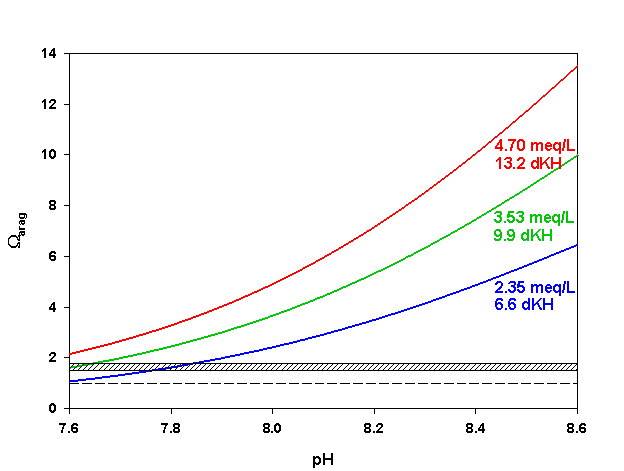
Figure 7. Effects of pH on Ωarag at three levels of alkalinity. Dashed line indicates threshold for aragonite dissolution. Hashed box indicates approximate threshold for hi-Mg calcite dissolution. Calculated using co2sys (Lewis and Wallace, 1998) assuming S = 35, T = 25 °C, P = 1 atm, and negligible total phosphate and silicate concentrations.
As we mentioned last month in our discussion of pH, however, it is not unusual to see a fair amount of pH variation on coral reefs over the course of 24 hrs. During the daytime photosynthesis removes CO2, raising pH in the water overlying the reef. The increase in pH shifts the inorganic carbon species toward CO32-, increasing Ωarag (Figure 7). Daytime pH may rise to 8.3-8.6, resulting in Ωarag as high as 5-7. At night the production of CO2 from respiration can reduce reef pH as low as 8.1-7.8, causing Ωarag to fall as low as 1.5-2.5 (Figure 7). Notice that these nighttime values for Ωarag are near or even slightly below those where we expect to begin to see dissolution of hi-Mg calcite. Dissolution of carbonates can and does happen on coral reefs today, especially at the lower pH values experienced at night.
Depending on how we manipulate Ca2+ concentration, alkalinity, and especially pH in our aquaria we can obtain values for Ωarag significantly above as well as below the range typical on a coral reef. We can produce conditions that favor the rapid precipitation of CaCO3 (significant supersaturation), and we can produce conditions that favor dissolution (undersaturation).
Given that there’s so much “extra” CaCO3 dissolved in sea water, we might expect that a lot of it should spontaneously precipitate out, just like in the experiment we discussed above. Spontaneous precipitation might be expected based on the thermodynamic solubility, but by and large it doesn’t happen, at least not quickly. Well, we might ask, why in the world not?
Calcium Carbonate Precipitation
Heat up a beaker of water and dissolve a large amount of table salt (NaCl) in it. Let the beaker cool down and you will have a supersaturated solution. If you then toss in a seed crystal, or anything else that salt crystals can grow on (a nucleation site) NaCl crystals will spontaneously precipitate out of solution. Scoop up a beaker of sea water next to a coral reef (supersaturated with respect to all three major polymorphs of CaCO3), toss in a seed crystal, seal it up, and put it on a shelf. You could wait months or even years all the while seeing very little happen. There must be something getting in the way of CaCO3 precipitation in sea water despite the fact that precipitation is thermodynamically favored.
One of the major obstacles to CaCO3 precipitation in today’s sea water is the high Mg2+ concentration of that water. Mg2+ exerts two distinct effects on CaCO3 precipitation. The first effect is an ion-pairing effect. Magnesium forms ion pairs with CO32- ions in solution. These ion pairs are short-lived, constantly forming and breaking apart, but they do affect the activity of CO32- in solution. An increase in Mg2+ concentration means that a larger proportion of the CO32- will occur as MgCO30 pairs, decreasing the activity of CO32-. In normal sea water, ~55% of the CO32- exists as ion pairs with Mg2+. Another ~10% pairs with Na+ ions and ~10% with Ca2+ leaving ~25% of the total as the free ion. By forming ion pairs with CO32-, Mg2+ does not make the precipitation of CaCO3 impossible, but it does slow it down significantly. Interestingly, by lowering the activity of CO32- in solution, Mg2+ allows more CaCO3 to dissolve than otherwise would. In this way, Mg2+ ions allow a large amount of CaCO3 to dissolve into sea water if that sea water becomes undersaturated with respect to aragonite and/or calcite, such as happens in the deep sea. Those Mg2+ ions also significantly slow down the rate of CaCO3 precipitation from sea water when that sea water becomes supersaturated, like in the shallow ocean. The ion-pairing between Mg2+ and CO32- slows down the rate of CaCO3 precipitation, but it alone is insufficient to explain why we don’t see more abiotic CaCO3 precipitation in sea water.
The second and more important effect that magnesium ions exert on CaCO3 precipitation is that they poison the surface of growing crystals. Magnesium ions are attracted to the carbonate ions in CaCO3 surfaces, much like calcium ions are. As they attach to these surfaces they can become incorporated into the growing crystal. Magnesium ions, while chemically similar to calcium ions (Mg is in the same period and directly above Ca on the periodic table), are the smaller of the two. Think of baseballs vs. softballs. While magnesium ions fit into the crystal lattice of CaCO3 well enough to be incorporated, they disrupt the pattern. Imagine building a brick wall: if all the bricks are the same size, it’s easy to construct the wall. Now imagine that every now and again a smaller brick is randomly inserted in place of a normal sized one, but the same amount of mortar is used to hold the bricks together. The wall would end up very misshapen in short order, and eventually would deviate so far from the original pattern it would be difficult to continue building at all. Magnesium ions disrupt the precipitation of CaCO3 in much the same way. They turn the growing surface of CaCO3 crystals into odd shapes where it is not easy for CaCO3 to precipitate. The higher solubility of MgCO3 as compared to CaCO3 also means that such crystals will more easily redissolve, inhibiting CaCO3 precipitation even if it is thermodynamically favored.
While magnesium ions disrupt the lattice structure of calcite, they fit well enough that they can be incorporated as a fairly large proportion of the crystal. Hi-Mg calcite is structurally the same as low-Mg calcite, except that many of the calcium ions have been replaced by magnesium ions, yielding to irregularities in the lattice structure. The ions in the aragonite lattice, however, are somewhat more widely spaced than in the calcite lattice. They are spaced widely enough that Mg2+ only rarely co-precipitates with Ca2+ in aragonite crystals. While some aragonite skeletons/shells contain more Mg2+ than others, none approach the magnesium content of hi-Mg calcite crystals. When the molar Mg/Ca ratio of a solution is < 1 low-Mg calcite tends to form preferentially. If the Mg/Ca ratio is increased then the calcite will incorporate progressively more and more Mg2+ into the crystals. At a Mg/Ca ratio between 1 and 2 we see the formation of primarily hi-Mg calcite. When the Mg/Ca ratio is increased above 2 we begin to see aragonite precipitation, along with hi-Mg calcite. As the Mg/Ca ratio is increased further still to 3, 4, 5 (or the 5.2 in today’s ocean) aragonite constitutes a larger proportion of the CaCO3 precipitated while the Mg content of the hi-Mg calcite continues to climb. If we raise the Mg2+ concentration high enough we can essentially inhibit calcite precipitation (as hi-Mg calcite) entirely. Aragonite precipitation, however, will continue to occur even at high Mg2+ concentration. Magnesium ions directly inhibit calcite precipitation by poisoning the growing crystal. Magnesium ions do not significantly affect aragonite precipitation, though low magnesium concentration favors the precipitation of calcite, outcompeting aragonite crystals for calcium and carbonate ions.
By maintaining the Mg2+ concentration in our aquaria near that in today’s sea water we can favor the precipitation of aragonite and hi-Mg calcite, the polymorphs of CaCO3 produced by nearly all of the organisms we keep in captivity. We can also minimize the rate of abiotic CaCO3 precipitation on pumps, heaters, and elsewhere in our aquaria. Sufficiently high Mg2+ concentration helps to maintain significant CaCO3 supersaturation in our aquaria, and the shallow ocean, and encourages rapid calcification and growth in the vast majority of calcifying organisms we might keep. Organisms that normally produce low-Mg calcite in today’s ocean either live in polar regions (low-Mg calcite is the favored polymorph at a temperatures < 2 °C) or do so in spite of the high Mg2+ concentration. That some organisms produce a thermodynamically unfavorable mineral for their shells/skeletons reminds us that biologically mediated calcification is fundamentally dependent upon the physiological capacities of the organisms performing the calcification, though environmental factors influence those capacities.
Conclusion
In this article we discussed the major interactions of the carbonate system in sea water. We began by exploring why sea water has the pH that it does. Seawater pH at any given moment is determined almost entirely by the interaction between total alkalinity and total CO2/dissolved CO2. The other parameters of the carbonate system, calcium and magnesium, do not directly affect pH. In order to appreciate why CaCO3 precipitates from sea water at all, we went next to the concept of saturation state, Ω. The polymorph of CaCO3 is a critical consideration in defining Ω though, so our discussion turned to CaCO3 mineralogy next. The organisms we keep in captivity generally produce aragonite or hi-Mg calcite, so the aragonite saturation state (Ωarag) is the one most useful to us. Calcium concentration and alkalinity tend not to vary much in nature at a given salinity, so variation in Ωarag is caused principally by the effects of varied pH on CO32- concentration. In captivity we can provide a much wider range of values for Ωarag because we are able to manipulate each of calcium concentration, alkalinity and pH. We can provide conditions that favor rapid CaCO3 precipitation, and conditions that favor dissolution. Lastly we saw that Mg2+ plays a critical role in CaCO3 dissolution and precipitation. The high concentration of Mg2+ in today’s ocean allows a large amount of CaCO3 to dissolve if sea water becomes undersaturated with CaCO3, but inhibits CaCO3 precipitation if sea water then becomes supersaturated. Magnesium ions help to keep CaCO3 supersaturated in our aquaria and in the shallow ocean by inhibiting abiotic precipitation of CaCO3. The high Mg2+ concentration in today’s sea water also favors the precipitation of aragonite and hi-Mg calcite over
low-Mg calcite, helping to favor the calcification and growth of the majority of the calcifying organisms we might keep in captivity. Next month we’ll discuss methods available to manipulate these parameters in aquaria and explore how different types of manipulations affect the entirety of the carbonate system.
References
- Lewis E, Wallace DWR (1998) Program developed for CO2 system calculations. ORNL/CDIAC-105. Carbon Dioxide Information Analysis Center, Oak Ridge National Laboratory, U.S. Department of Energy, Oak Ridge, Tennessee.
- Millero FJ (2006) Chemical Oceanography, Third Edition. Taylor and Francis Group, Boca Raton, FL.
- Mucci A (1983) The solubility of calcite and aragonite in seawater at various salinities, temperatures, and one atmosphere total pressure. Am J Sci 283:780–799.
- Pearson PN, Palmer MR (2000) Atmospheric carbon dioxide concentrations over the past 60 million years. Nature 406:695–699.
0 Comments