

Abstract
The purpose of this study was to investigate a method to more accurately determine the output flows of several aquarium propeller pumps. To complete this investigation, a test setup was constructed in a 350 gallon aquarium tank using a Sontek 10-MHz Acoustic Doppler Velocimeter for data acquisition. The velocity profile of the pump exit flow was measured at a distance of one diameter downstream from the output of the pumps and used to determine the volume flow rate output. The results of this investigation reveals that there can be large variability between the manufacturer’s advertised flow rates for propeller driven pumps and the flow rates measured by this method. The results suggest that a standardized approach to measuring flow should be created to better enable manufacturers to more accurately advertise the correct flow rates so that consumers can choose the appropriate pump for their aquarium.
Flow in the Aquarium
Sufficient water movement in aquariums is known to be an important component for animal health and long term success. In general, most reef hobbyist attempt to maximize the water movement within their aquarium (flow rate) using pumps, power heads, or wave devices while minimizing the maximum velocity of the water “hitting” sessile animals. This prevents shearing off of tissue and disturbing the health of corals. The flow rate is defined as the amount or volume of water moved per unit of time and is usually provided in units such as gallons per hour or liters per hour.
However there are no simple rules on how to adequately quantify the amount and type of water motion needed for aquarium success. Reasons for this include the lack of a detailed data and real understanding of the needed water movement or type of movement necessary for specific animals. In general, the amount of water motion for corals has been linked to the location of specimens relative to the reef zone (such as fore reef, reef flats, lagoon, etc). However in reality the water motion in the ocean is very chaotic both in short (seconds, minutes) and long (hours, days and longer) time scales. In an aquarium the amount of achievable flow at any point is further complicated and impacted by both aesthetic (non-living) and living (such as coral) structures, placement of pumps, and tank walls; all of which add friction, change flow direction and constrain or limit water movement. Also any structure in the path of water flow can induce change in flow directions, secondary flows, momentum losses, unsteadiness and turbulence.The aquarium industry characterizes the pumps using the flow rate – amount of water moved per unit of time (eg. Gallons/hr). However, the more accurate definition of volumetric flow rate is ” the volume of fluid which passes through a given surface area per unit time” This definition indicates that there is a velocity component to the flow. For a fixed surface area, the volumetric flow rate can be increased or decreased by changing the flow velocity. Also, a fixed flow rate can be achieved by increasing the velocity and reducing the surface area or by decreasing the velocity and increasing the surface area.Given an area A, and a fluid flowing through it with uniform velocity V with an angle away from the perpendicular direction to A, the flow rate is:
Q = (V)(A) cos θ (1)
In the special case where the velocity is perpendicular to A,
Q = (V)(A) (2)
In general, the flow velocity at any location in the ocean (or in the aquarium) can be in any direction and can be defined by a vector or
 (3)
(3)
Since the direction and magnitude of the velocity may change in time, the water velocity can also be defined by
 (4)
(4)
where  is the mean velocity component of the fluid and V’ is the unsteady or time-varying component . The magnitude and direction of the unsteady component, V'(t) is a function of time. The unsteady component can also be sub-classified as deterministic (such as periodic or coherent variations in water movement due to waves or wakes from the rotating propeller blades) or non-deterministic (random motion or turbulence). Turbulence is initiated by shear or gradients in flowing water and is characterized by chaotic mixing of the water through large scale eddies which spawn ever smaller scale eddies.
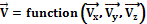
In the aquarium, water movement is typically achieved using powerheads or pump driven return pipes and closed loop circuits. The outlet portion of each of these devices results in the generation of a submerged jet similar to what is shown in Figure 1 for a simple submerged turbulent jet. Submerged jets are jets of water that flow into a reservoir (tank) of water. Contrary to common aquarium myth, in most cases, except possibly the smallest powerheads, the jet is turbulent and not laminar. Also, as will be shown in this paper, the exit flows from propeller driven pumps are much more complicated than a simple jet shown below.
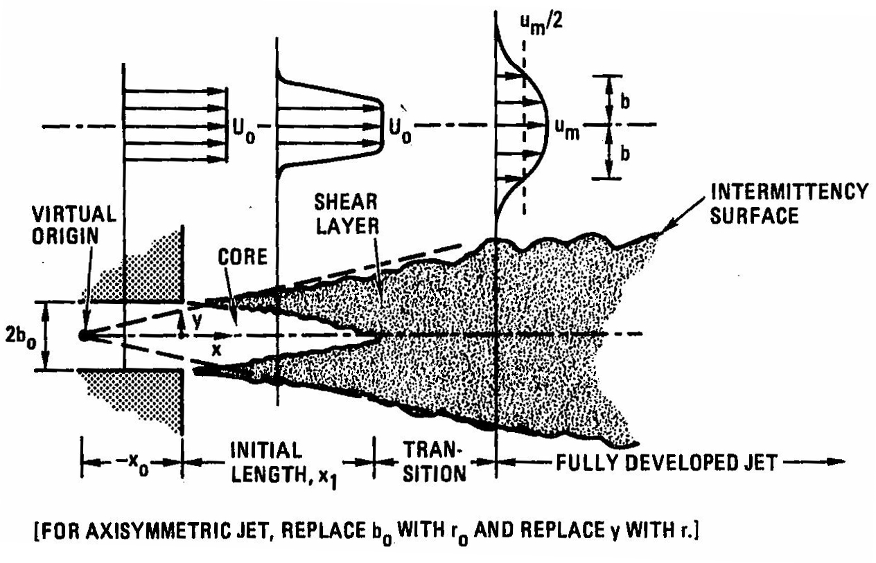
Figure 1. Schematic of simple turbulent jet [1]
Introduction
The use of propeller bladed pumps/powerheads for water movement in the aquarium industry has expanded significantly in the past few years with the advent of DIY, retrofit kits, and specific commercial lines. The first propeller pump available to reef aquarist consumers was created by Jimmy Chen in 2002 and sold as a retrofit kit to be installed on a Little Giant submersible pump [2]. While providing high flow rates with minimal power consumption, this product did not feature the benefit of long term research and development and was plagued by failures. tunze unvieled the first widely available commercialized propeller pumps at Interzoo in May 2002 branded as the “Tunze Stream.” The synchronous models of Stream were available at retail in July 2002 and the controllable models followed in November. They also offered brushless DC models which were capable of speed control through their own proprietary controller.
In 2005 EcoTech Marine introduced a through-the-glass magnetically coupled aquarium pump, using a brushless DC, controllable motor. More recently, Hydor introduced their Koralia line of propeller pumps and made available controllable versions as well. The Hydor line of controllable powerheads is distinctly different from the tunze and EcoTech Marine products because it utilizes low voltage AC current to drive the pumps and the controllers use frequency modulation to change the speed. The major difference of these two approaches is that brushless DC pumps are typically more expensive but their controllers are relatively inexpensive, whereas low-voltage AC pumps are more economical however their controller is expensive to produce. Generally, brushless DC pumps are capable of more precise rpm changes to enable flow augmentations such as pulsing for waves generation.
The objective of the current experiment was to investigate a more accurate method to determine the volumetric flow rates for widely available models of propeller pumps. The advantage of propeller pumps is that they are capable of moving large volumes of water at very low pressures with minimal power consumption. Some DIY methods of measuring the flow rate of small pumps include timed bag filling experiments, pumping from one reservoir to another and placing the powerheads in a constrained systems (inlet or exit piped) with a flow meter. These types of tests however, can impart unrealistic hydrodynamic loads on the propeller pumps by altering the inlet and/or exit flows in ways that are not typically seen in our aquarium set ups. Adding piping and other constraints such as bags on the exit jet may impart back-pressure that can affect the pump’s performance. These DIY methods add additional blockage (similar to covering the exit jet or inlet grating) which negatively reflects the true flowrate of the pump. In addition, the pump exit jet flow tends to expand radially as it exits the nozzle as shown in the Figure 1. Any intrusive method (such as a bag, added piping, increased pressure head between reservoirs) adds momentum and friction losses not accounted by most measurement methodologies. Therefore more sophisticated methods must be employed to obtain accurate flow readings from propeller driven pumps. An experimental method was developed incorporating acoustic Doppler velocimetry (ADV) technology, which has been used to measure open channel flow. The advantage of this methodology is that it is nearly non-intrusive and does not apply backpressure to the pump. It also measures the flow velocities directly in contrast to diffusion/dissolving methods which only infer flow rates [3].
The pumps included in this study are listed in Table 1 along with their manufacturer’s advertised flowrate. Due to the expense of some of these products and constraints on the budget, every product on the market could not be included in this evaluation. The study was restricted to the following list of pumps shown in Table 1.
| Pump | Advertised Output Flow (Gallons/hr) |
|---|---|
| Aqueon 2400 | 2400 |
| Coralife CP 2900 | 2900 |
| Ecotech Marine MP-10 | 1575 |
| Ecotech Marine MP-40 | 3200 |
| Ecotech Marine MP-60 | 7500 |
| Hydor Koralia 5 | 1650 |
| Hydor Koralia 6 | 2200 |
| Hydor Koralia 7 | 2700 |
| Hydor Koralia 8 | 3250 |
| Maxijet 1200 | 295 |
| tunze 6105 | 3434 |
| tunze 6205 | 5811 |
| tunze 6305 | 7925 |
The majority of the pumps included in this test cater to the high-end saltwater aquarium market. A less expensive traditional impeller driven Maxijet 1200 powerhead was included in this test as a comparison to propeller pumps.
Figure 2. Division of flow based on radial position
Theory
Because these propeller based aquarium pumps operate between two fluid reservoirs that are at the same pressure, one cannot simply displace water from one reservoir to another without adversely affecting the accuracy of the measured volume flow rate. For this reason, a velocity measurement of flow is needed to determine the true volume flow rate through the pump. A single velocity measurement is not sufficient for propeller pumps since the flow velocity varies across the large diameter cross section of the exit nozzle. To accurately measure the velocity of the flow across the entire output profile, several sample measurements were taken at locations ranging from the very outside of the flow jet to the center of the flow jet. For the purpose of this experiment, the flow was divided into n distinct regions, illustrated in Figure 2.
After measuring the flow velocity in these regions, the subsequent volume flow rate of the region can be found using
VFRi = Vi*Ai (5)
where, VFRi is the volume of water flowing per unit time through the incremental area Ai at velocity Vi . This calculation can be repeated over the velocity profile to yield the total volume flow rate of the system. This idea can be expressed as
VFRs = Σ Vi * Ai. (6)
The area of each region can be calculated using
Ai = π * (ri2-r(i-1)2). (7)
This type of calculation is known as a Reimann Sum, and is used to approximate real-world integration. The accuracy of this method depends greatly on the number of iterations completed.
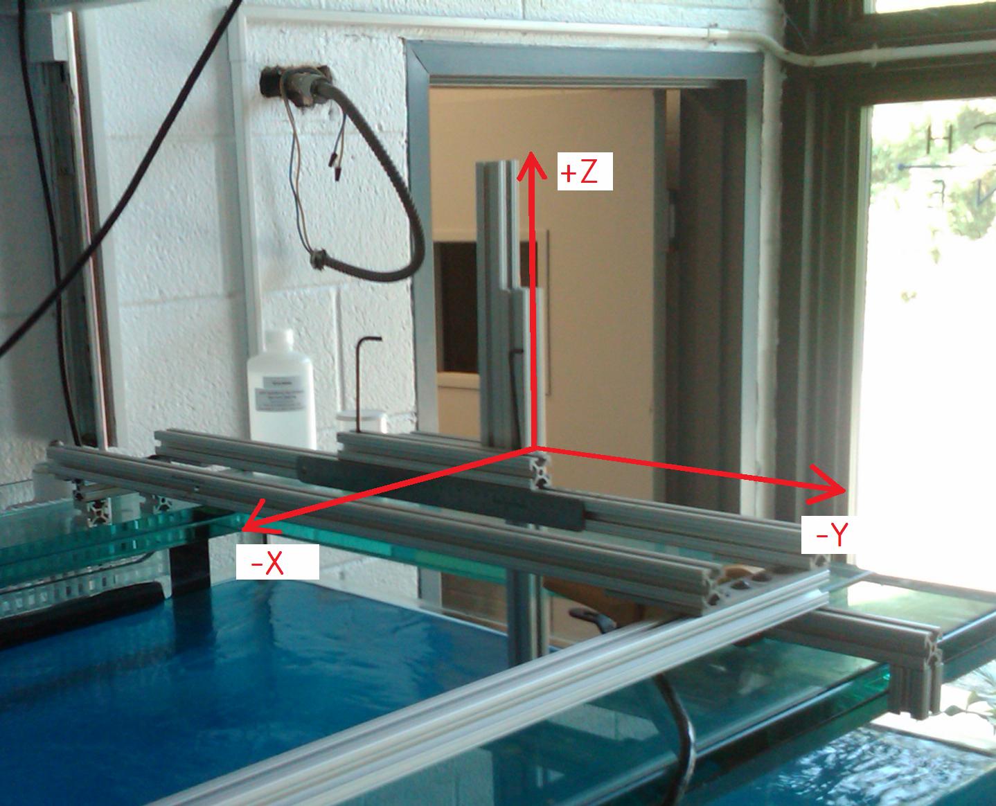
Figure 3. Scaffolding support structure for ADV positioning
Experimental Apparatus
For this experiment, a test setup needed to be developed that would accurately measure the velocity of water flow over a series of points across the flow profile. To accomplish this task, a Sontek 10-MHz Acoustic Doppler Velocimeter was selected for its ability to measure open-channel flow in a volume of water as small as 0.25 cc. The ADV selected also had the capability of measuring 3-Dimensional flow. Table 2 is taken from Sontek’s literature for the 10 MHz ADV used.
The ADV that was used to collect the velocity measurements was positioned using an extruded aluminum scaffolding system shown in Figure 3. The system was designed to be adjustable in the three dimensions shown, labeled X, Y, and Z. The vectors shown correspond to the ADV measurements taken for the X, Y, and Z directions.
To accurately measure the position of the ADV over the course of each trial, the scaffolding structure in Figure 3 was fitted with Wixey Model WR510 digital positioning gauges on both the Z and the Y axes. The specifications for the gauges used are shown in Table 3.
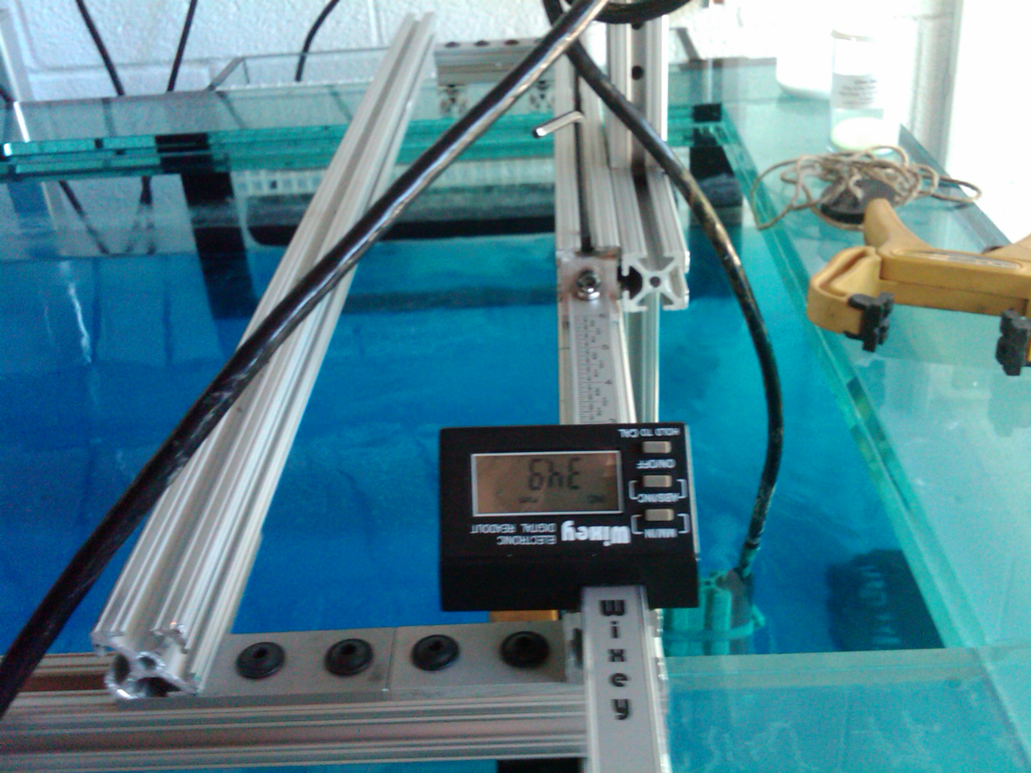
Figure 4. Integration of digital positioning gauges into scaffolding structure
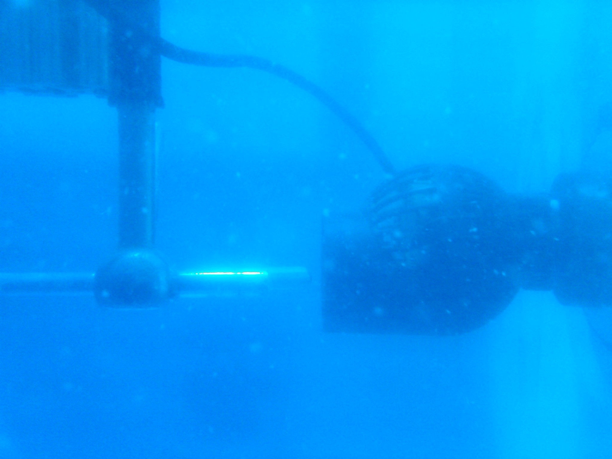
Figure 5. Initial positioning of the ADV during testing
| Wixey Model WR 510 | |
|---|---|
| Resolution: | Decimal = .005 in. |
| Fraction = 1/32 in. | |
| Metric = 0.1 mm | |
| Accuracy: | Decimal = .0025 in. |
| Fraction = 1/500 in. | |
| Metric = .05 mm | |
Figure 4 shows the setup of the positioning and integration of one of the gauges used. This test setup allowed for accurate recording of the position of the ADV to within 0.05 mm, as listed in the specifications. Because positioning in the X direction was less critical, a tape measure was used to position the ADV at approximately one diameter downstream from the face of the pump, +/- 1/32nd of an inch.
Figure 5 shows the final ADV positioning for testing of the tunze 6305. As shown in the figure, the ADV is positioned at the centerline of the pump face and one diameter downstream from the face.
Figure 5 also shows the particulate matter that was suspended in the tank for the duration of testing. These particulates were the seeding material provided by Sontek in order to increase the signal-to-noise ratio returned by the velocimeter.
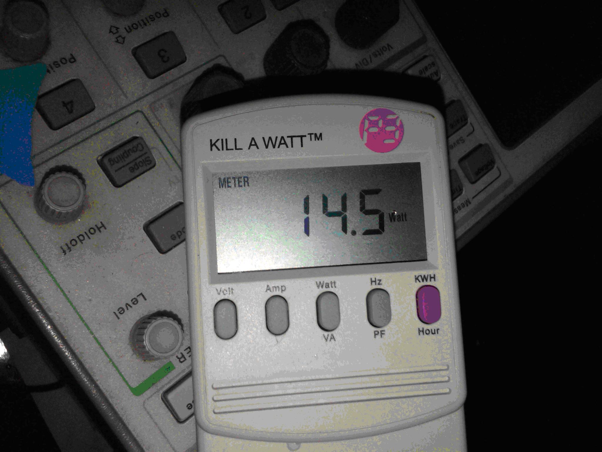
Figure 6. Watt meter used in testing
Besides the velocity components and standard deviation of the axial velocity, the power consumption and the rotational speed of each pump were recorded. The power consumption was monitored through a wattmeter which is shown in Figure 6. The rotational speed of each pump was determined using the strobe tachometer shown in Figure 7. Figure 8 shows the tachometer in use while testing the Coralife CP 2900.
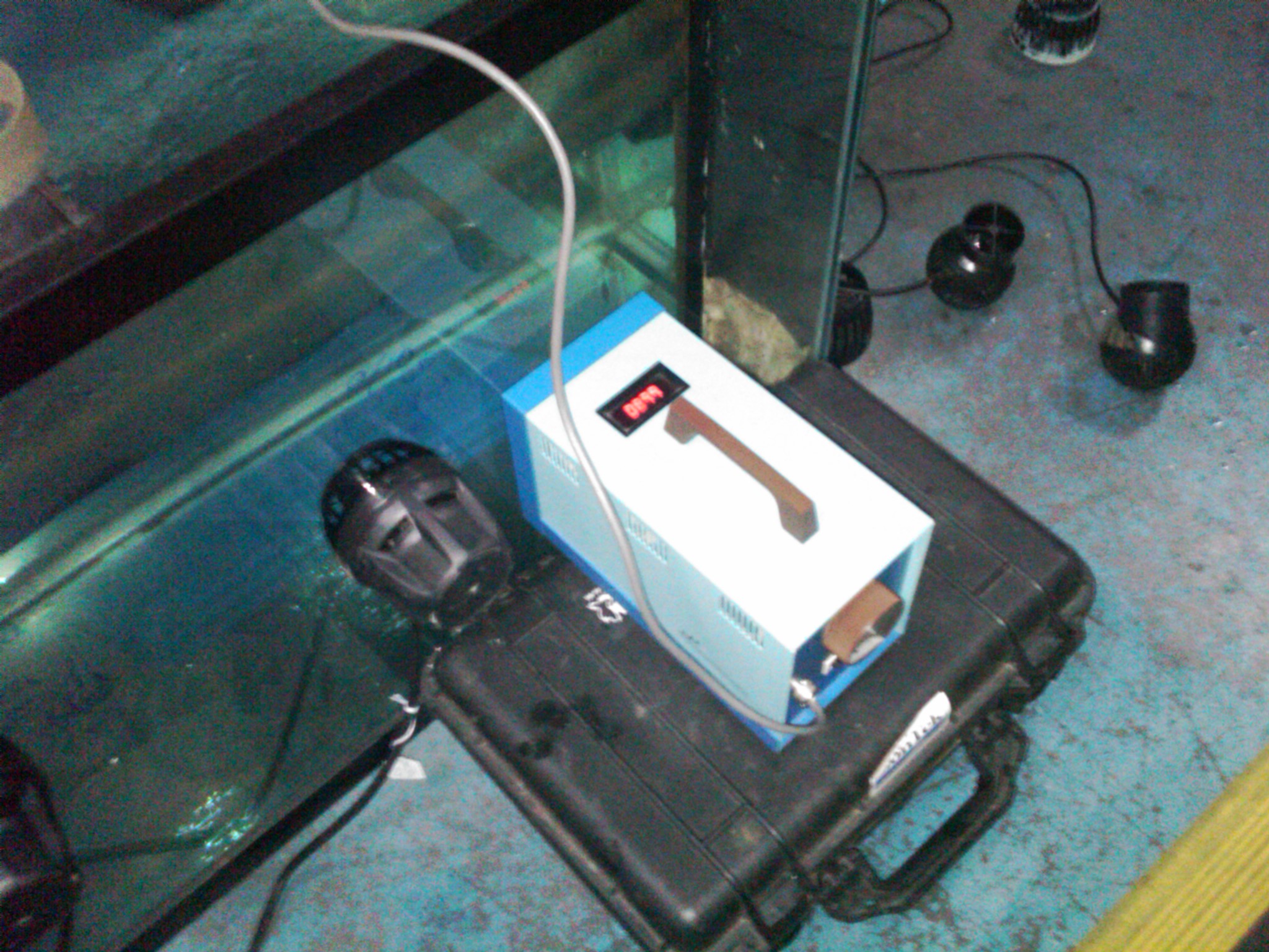
Figure 7. Strobe tachometer used in testing
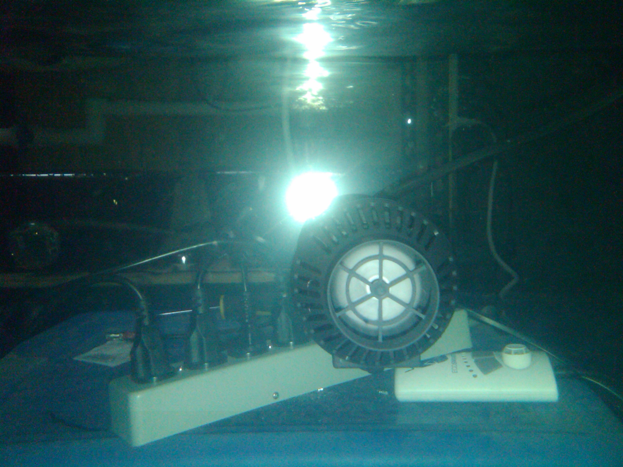
Figure 8: Coralife pump as seen under strobe lighting
Test Procedure
Before testing could begin on any of the pumps, an appropriate measurement time duration needed to be established to ensure that enough samples were taken to accurately represent the measured flow velocity and minimize measurement bias. To determine this duration, a value of the turbulence intensity was determined for several trials of differing time durations. The turbulence intensity FT is calculated using Equation 11, where is the standard deviation of the axial velocity and Vavg is the mean of the sample velocity.
FT = σ / Vavg (8)
The turbulence intensity is a value representing the degree of unsteadiness or fluctuations in the measured flow field. An ideal steady flow with absolutely no fluctuations would have a turbulence intensity value of zero. When measuring unsteady flows, care must be taken to ensure that the fluctuations are accounted for and do not lead to temporal biasing of the mean velocity measurements. Theoretically, the mean velocity and turbulence intensity values will approach constant values as the sample time is increased to infinity. The reason for this is that as sample time is increased, any temporal bias in the measurement will be reduced.
During the test, two trials were averaged at various time intervals to produce the data shown in Table 4. The data was then plotted in Figure 9 to locate the “shoulder” of the curve, or the point that would produce reliable and accurate velocity data.
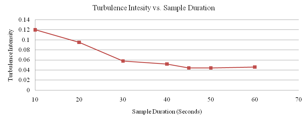
Figure 9. Turbulence Intensity plotted for various time durations
| Time (sec) | Sigma (ft/sec) | V (ft/sec) | FT |
|---|---|---|---|
| 0 | 0.30 | 2.5 | 0.120 |
| 20 | 0.21 | 2.2 | 0.095 |
| 30 | 0.14 | 2.4 | 0.058 |
| 40 | 0.12 | 2.3 | 0.052 |
| 45 | 0.11 | 2.5 | 0.044 |
| 50 | 0.11 | 2.5 | 0.044 |
| 60 | 0.11 | 2.4 | 0.046 |
As shown in Figure 9, the point at which the turbulence intensity curve leveled off was found to be about 45 seconds. This duration was determined adequate to represent the velocity data for the pumps. For the extent of the test, velocity samples were taken using this time duration for sampling at each location.
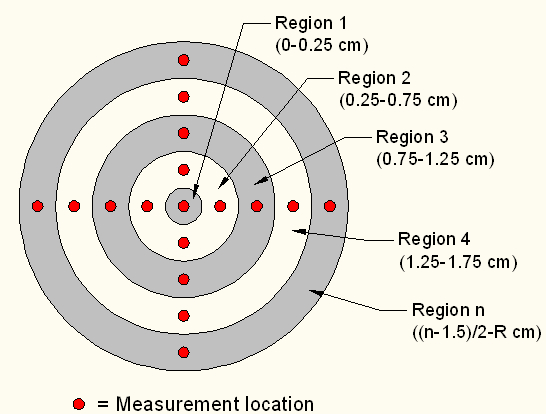
Figure 10. Illustration of velocity measurement locations
With the time of each sample established, flow testing on the pumps could begin. The output nozzle diameter was measured for each pump and recorded for later use. Flow testing was broken down into two sets of trials for each pump: a horizontal set and a vertical set. The two data sets allowed the flow to be broken into four quadrants, providing a more accurate measure of the entire velocity profile. The data points taken are shown in Figure 10.
To begin taking data, the ADV was positioned such that the sampling volume of the measurement corresponded to the center of the pump output and was located one diameter downstream of the nozzle, as illustrated in Figure 5. The ADV was first positioned well outside the range of the flow, which was defined as a stagnant, or near zero, X velocity. The velocimeter was then moved in the positive Y direction across the velocity profile in 5mm increments until a non-stagnant X velocity was observed. Velocity measurements were then recorded for successive 5mm increments for the entirety of the profile until a stagnant velocity was reached at the corresponding location on the opposite side of the flow jet. This process was repeated moving the ADV vertically to achieve the measurements shown in Figure 10.
The raw data taken during the testing needed to be corrected before it could be used to calculate the volume flow rate. To begin, the velocity measurements taken from the velocimeter were in component form. The three velocity components (along the X, Y and Z axis) needed to be combined through vector addition in order to produce the final velocity measurement for the given location. This process is described through Equation 12, where Vtotal is the combined velocity, and Vx,y,z are the individual component velocities. This is an important step as the rotating propeller blades in many of the tested designs swirl the flow in a screw like fashion. The exit jet also expands as it leaves the pump. A simple one component velocity measurement may underestimate the actual water velocity.
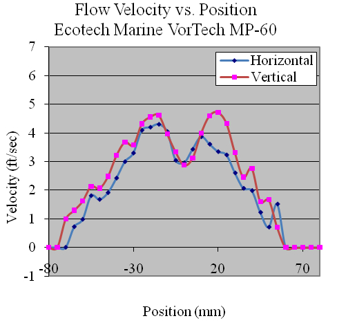
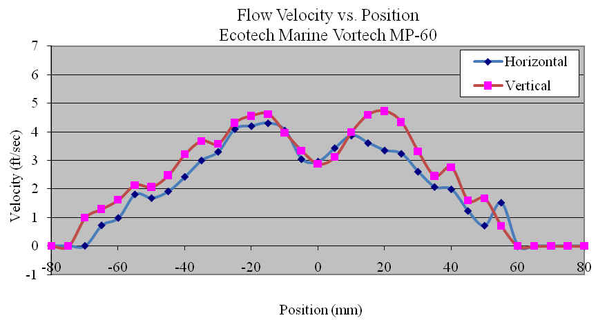
Figure 11. Velocity Profile of Ecotech Marine vortech MP-60
Vtotal = (Vx2 + Vy2 + Vz2)1/2 (12)
The next modification to the data was made to “center” the measured points. This process was done to ensure that the velocity measurements taken matched up correctly to their radial location used in the flow calculation. Centering the data involved a set of criteria described below:
- If the data contained an obvious flow deficit (“void”) which represented the center of the propeller, the data was centered such that the void was assigned a radial position of 0 mm.
- If the measured data did not contain an obvious flow deficit the data was centered symmetrically over a radial position of 0 mm.
To measure the rotational speed of the pumps, a small mark was painted on one side of the propeller, and the pump was turned on and set to the maximum speed. The strobe tachometer was positioned outside the aquarium facing the pump. The speed of the tachometer was adjusted until the mark on the propeller appeared stationary, and the RPM value displayed was recorded.
To measure the power consumed by each pump, the power source was run through the wattmeter shown in Figure 6. There was often a “settling” period observed where the pump initially drew slightly higher wattages, so the power value was recorded after taking the velocity measurements.
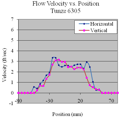
Figure 12. Velocity Profile of tunze 6305
One exception made to this procedure was the measurements made on the MaxiJet 1200. This pump had an output diameter of less than ½”, making measurement difficult at one diameter downstream. To compensate for the small output radius and ensure enough data points were taken, the ADV was positioned 1″ downstream from the face of the pump. Due to the lack of a visual propeller on the MaxiJet, the pump speed was not measured.
Results
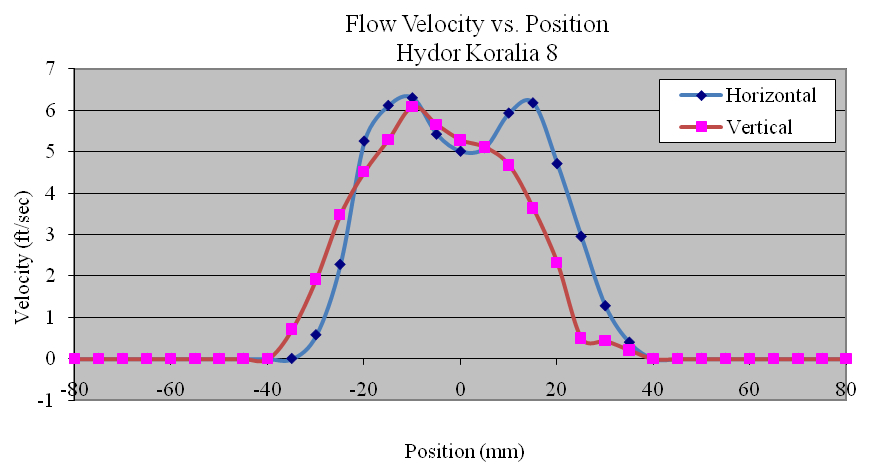
Using the data collected, the flow profiles of the pumps was computed in the Z (vertical) and Y(horizontal) directions. The majority of the pumps tested produced nearly symmetric velocity profiles. Figures 11, 12 and 13 show the Ecotech Marine MP-60, the tunze 6305, and the Hydor Koralia 8, respectively, which are examples of pumps that exhibited somewhat symmetrical flow fields. These figures show the results of both the horizontal and the vertical data sets for each pump. In these examples, it is seen that the MP-60 and tunze 6305 produced a broad and comparably gentle flow, where the Koralia 8 produced a more concentrated jet with a higher peak velocity. The flow profiles for all the pumps is presented in Appendix 2. The reader should note the differences in complexity of the flow generated by the propeller generated pumps compared to that of a traditional impeller driven powerhead like the Maxijet 1200 (see Figure Appendix 2.7). The complexity of their exit flow field that makes simple single point measurement methods unreliable in determining rated flow rates.
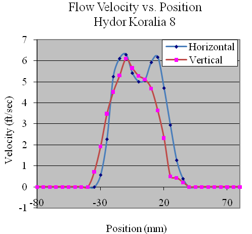
Figure 13. Velocity Profile of Hydor Koralia 8
Uncertainity and Error
While the Sontek specifications state a measured accuracy of +/- 1% of the reading, in actual situations this error will be higher. There are several sources of error and uncertainity that contribute to the flow calculations, some of which are listed below
- Approximations used for integration depend on the granularity of data and number of points sampled
- Unsteady nature of the flow field, due to blade wake passing, asymmetric or blocked inflow, inlet and exit grill interactions, ADV vibrations, etc.
While all the associated uncertainties are difficult to quantify without detailed analysis and huge investments in time and effort, based on our experience with flow measurements it is reasonable to expect that the error range of the calculated volumetric flow rates to be limited to 5-7% of the reported values.
Based on these flow profiles, the volumetric flow rate was calculated. The results are presented in Table 5. The column on the far right labeled “% Change from Manufacturer’s Claim” is a comparison between the calculated experimental flow and the manufacturer’s stated maximum output flow. This calculation is expressed by
 (13)
(13)
Table 5 represents the data such that a positive change indicates an increase in the observed flow from the manufacturer’s claim and vice versa. The data is shown graphically in figure 15.
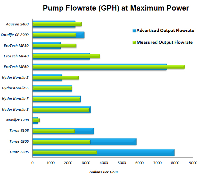
Figure 14. Comparison of Advertised Output Flowrates with Measured Output Flowrates
| Pump | Pump Speed (RPM) | Power Use (Watts) | Calculated Flow (Gal/hr) | % Change of Mean from Manufacturer’s Rate |
|---|---|---|---|---|
| Aqueon 2400 | 3600 | 14.2 | 2744 | 14.30% |
| Coralife CP 2900 | 3600 | 18.8 | 2437.2 | -16.00% |
| Hydor Koralia 5 | 3600 | 22 | 2597.59 | 57.43% |
| Hydor Koralia 6 | 3600 | 21.8 | 2205.6 | 0.30% |
| Hydor Koralia 7 | 3600 | 12 | 2659.1 | -1.50% |
| Hydor Koralia 8 | 3600 | 18 | 3188.3 | -1.90% |
| MaxiJet 1200 | Unknown | 20.7 | 405.7 | 37.50% |
| tunze 6105 | 3250 | 24 | 2358.2 | -31.30% |
| tunze 6205 | 3160 | 45 | 3234 | -44.30% |
| tunze 6305 | 3060 | 48 | 3597.3 | -54.60% |
| vortech MP-10 | 3270 | 19.8 | 2460.3 | 56.20% |
| vortech MP-40 | 2440 | 29 | 3781.2 | 18.20% |
| vortech MP-60 | 2100 | 53 | 8509.8 | 13.5% |
Another metric that could be use to evaluate the pumps is the Flow Efficiency, measured as the ratio of measured flowrate to actual power consumed. Table 6 and Figure 15 summarizes the flow efficiencies in units of GPH/watt. As shown, the pumps are broken into three different categories: AC (non-controllable), ACC (controllable), and DC (controllable). While the AC models offer better flow efficiencies, they do not offer the flexibility of output modification or advanced programming. The highest efficiency for the ACC pumps was the Hydor Koralia 7 and for the DC pumps was the Ecotech Marine vortech MP-60.
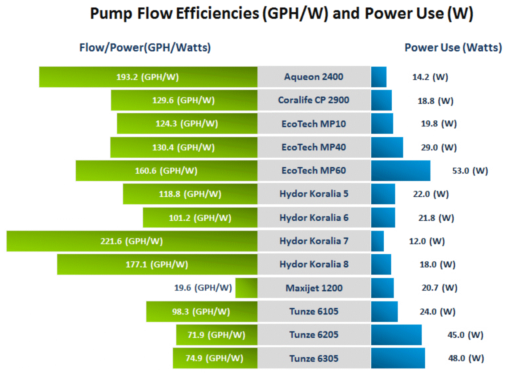
Figure 15. Flow Efficiency of the Pumps Tested
| Pump | Flow/Power (GPH/watt) | Power Type (AC/DC) |
|---|---|---|
| Aqueon 2400 | 193.2 | AC |
| Coralife CP 2900 | 129.6 | AC |
| Hydor Koralia 5 | 118.8 | ACC |
| Hydor Koralia 6 | 101.2 | ACC |
| Hydor Koralia 7 | 221.6 | ACC |
| Hydor Koralia 8 | 177.1 | ACC |
| MaxiJet 1200 | 19.6 | AC |
| tunze 6105 | 98.3 | DC |
| tunze 6205 | 71.9 | DC |
| tunze 6305 | 74.9 | DC |
| vortech MP-10 | 124.3 | DC |
| vortech MP-40 | 130.4 | DC |
| Vortech MP-60 | 160.6 | DC |
Conclusions
A standard method for evaluating flow rates of pumps using ADV was developed, and applied to measurement of flow of several popular aquarium propeller pumps. Data obtained during this study shows that the generated flow field is more complex than a simple submerged jet and therefore single point measurements may not accurately represent the flow rate. After the completion of this experiment, it is clear that there is a difference between many of the measured results and their manufacturer’s advertised performance. While most aquarium manufacturers are within a reasonable range of their claimed flows, there were some notable exceptions. As shown, measured values of volume flow rate for the Aqueon, MaxiJet, and EcoTech Marine models were generally higher than advertised flow outputs. The Hydor 6, 7, and 8 were measured to within 2% of the manufacture specifications. The Hydor 5 and vortech MP-10 both presented an anomaly in that they produced 55-60% more flow than claimed. In fact, the Koralia 5 that was tested produced significantly more flow than the Koralia 6, and almost matched the output of the Koralia 7. The reason for this difference in claimed and experimental flow measurements is unknown.
On the other hand, for the tunze units’ measured flow rates were consistently under the advertised flow rates on the models tested. In the case of the tunze 6305, the measured flow was less than half that of the manufacturer’s claimed flow. Further investigation may be needed to determine how this manufacturer originally developed the advertised flow rates of each of its models (see Addendum).
Another conclusion that can be drawn from this experiment is that there is a wide range of flow efficiencies shown. The flow efficiency, or unit of flow observed per unit of power consumed, varies greatly from manufacturer-to-manufacturer and model-to-model. The flow efficiency values are presented in Table 6.
Hobbyists have seen significant advancements in the range of aquarium circulation pumps available over the past decade. While all manufacturers provide a flow rate for the pumps, it is not clear what methods have been used to arrive at the numbers. Further, different manufacturers may use different methods. We have presented a standard method that we hope can be adopted by the manufacturers thus enabling a more accurate and verifiable approach.
Addendum
On completion of the study, the paper was sent to tunze and Hydor prior to this publication. Based on these results, tunze conducted its own independent tests on the Tunze pumps and have confirmed our results. On further discussion with Tunze we do not feel the errors were deliberate attempts to mislead, but rather their misguided faith in theoretical calculations that often do not translate well into real world application and use. In light of these finding tunze is working to remedy the situation. For any resolution on how tunze will address this please refer to Tunze’s website for more information.
Acknowledgment
We would like to thank EcoTech Marine for providing the large aquarium and renting the equipment needed for the study. The work was performed under the technical guidance and consultation with Bill Straka and Sanjay Joshi of Penn State University. The data was collected by Mike Sandford during his summer internship at EcoTech Marine.
References
- Blevins, R. D., Applied Fluid Dynamics Handbook, Van Nostrand Reinhold Co., New York, 1984.
- Harker, Richard. “Product Review: Propeller Pumps In The Aquarium.” Advanced Aquarist. Pomacanthus Publications, LLC. Web., http://www.advancedaquarist.com/2002/6/review.
- Riddle, Dana. “”Feature Article: Measuring Water Movement in Your Reef Aquarium for Less Than $100.” Advanced Aquarist. Pomacanthus Publications, LLC. Web., http://www.advanceda quarist.com/2011/1/aafeature.
- Taylor, John R. “Chapter 3.” An Introduction to Error Analysis: the Study of Uncertainties in Physical Measurements. Sausalito, CA: University Science, 1997. Print.
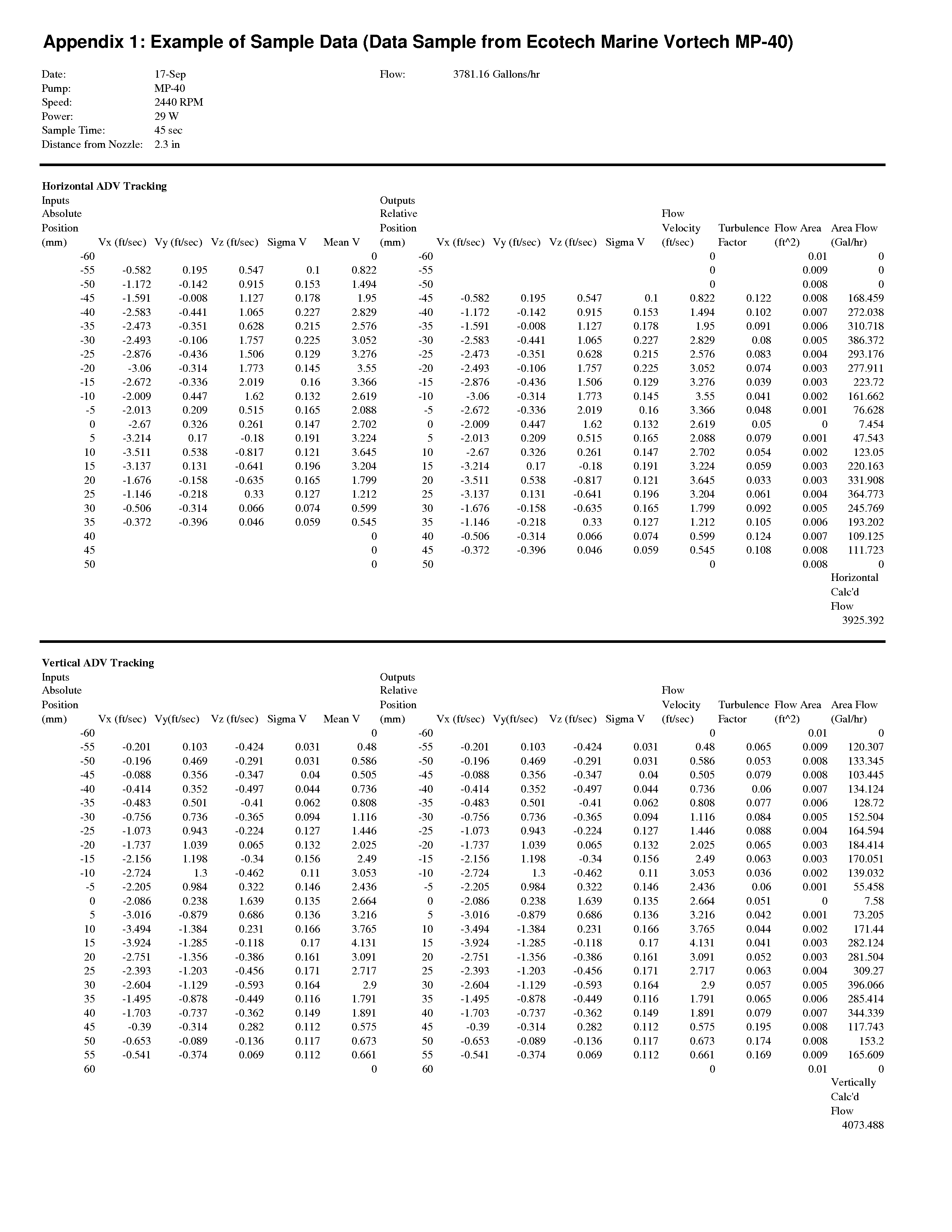
Appendix 1: Example of Sample Data (Data Sample from Ecotech Marine Vortech MP-40)
Editor’s note: The original article contained an embedded table that was to be displayed in-line with the article. Due to width constraints, we have instead converted this data into an image and are providing the data as an Excel spreadsheet and Adobe PDF.
Appendix 2: Plots of Velocity Profiles
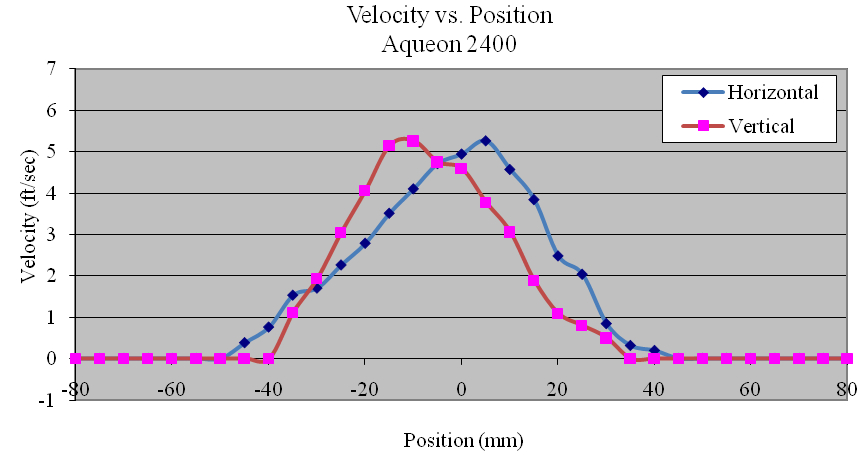
Appendix 2.1. Velocity profiles of the Aqueon 2400
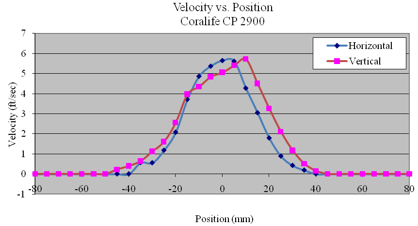
Appendix 2.2. Velocity profiles of the Coralife CP 2900
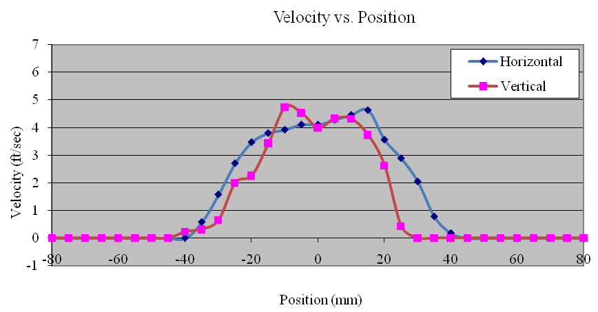
Appendix 2.3. Velocity profiles of the Hydor Koralia 5
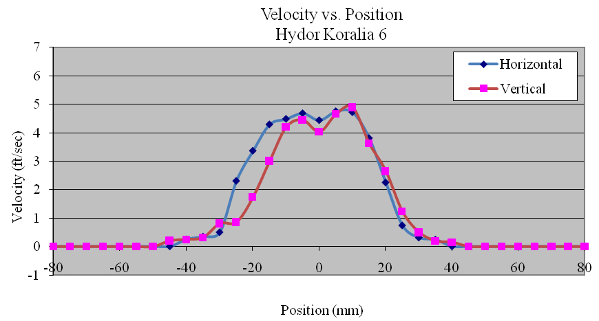
Appendix 2.4. Velocity profiles of the Hydor Koralia 6
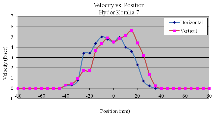
Appendix 2.5. Velocity profiles of the Hydor Koralia 7
Appendix 2.6. Velocity profiles of the Hydor Koralia 8

Appendix 2.7. Velocity profiles of the MaxiJet 1200
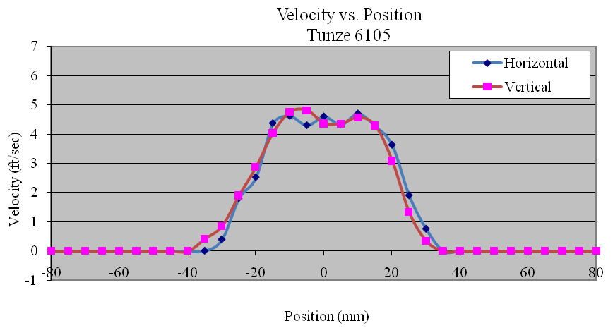
Appendix 2.8. Velocity profiles of the tunze 6105
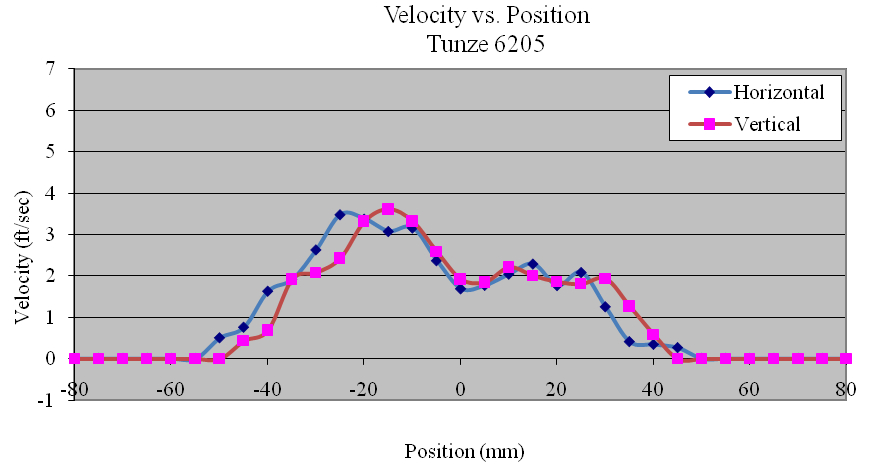
Appendix 2.9. Velocity profiles of the tunze 6205
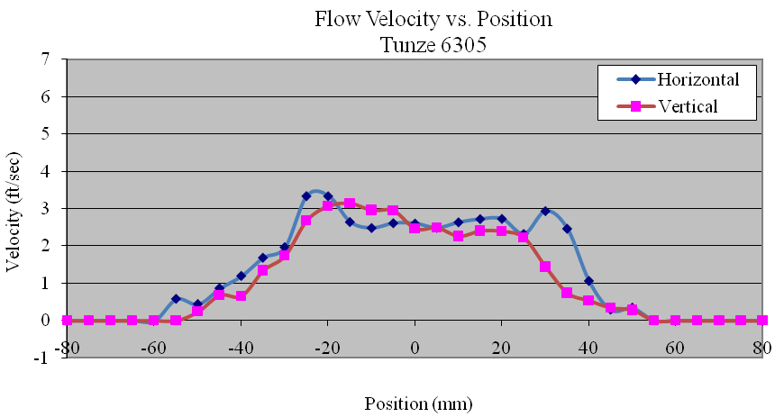
Appendix 2.10. Velocity profiles of the tunze 6305
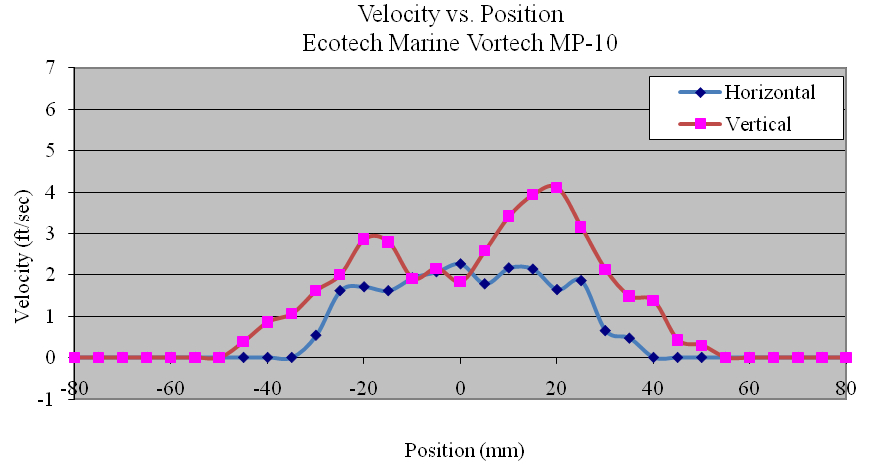
Appendix 2.11. Velocity profiles of the Ecotech Marine Vortech MP-10
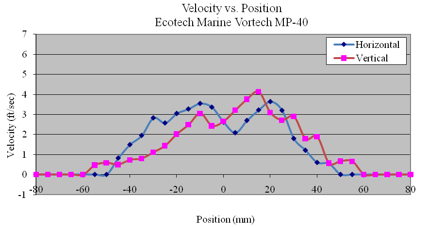
Appendix 2.12. Velocity profiles of the Ecotech Marine Vortech MP-40
Appendix 2.13. Velocity profiles of the Ecotech Marine Vortech MP-60
0 Comments