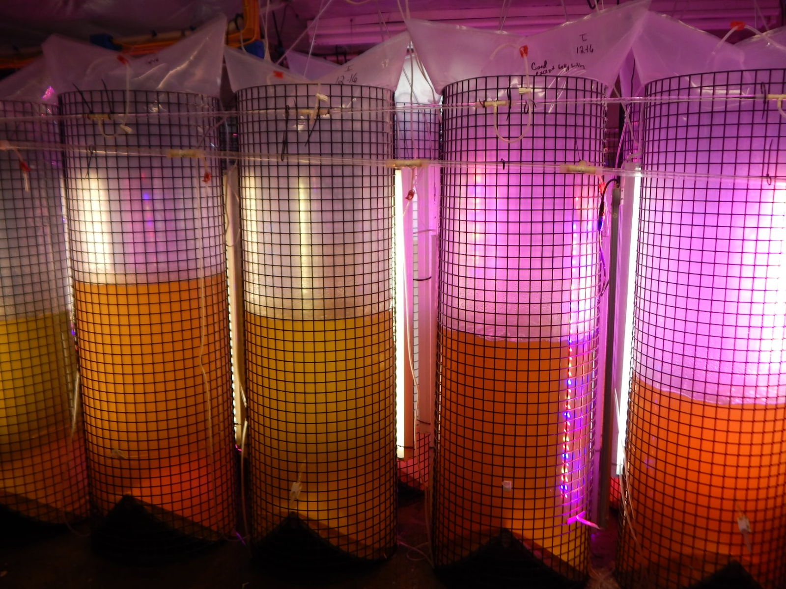
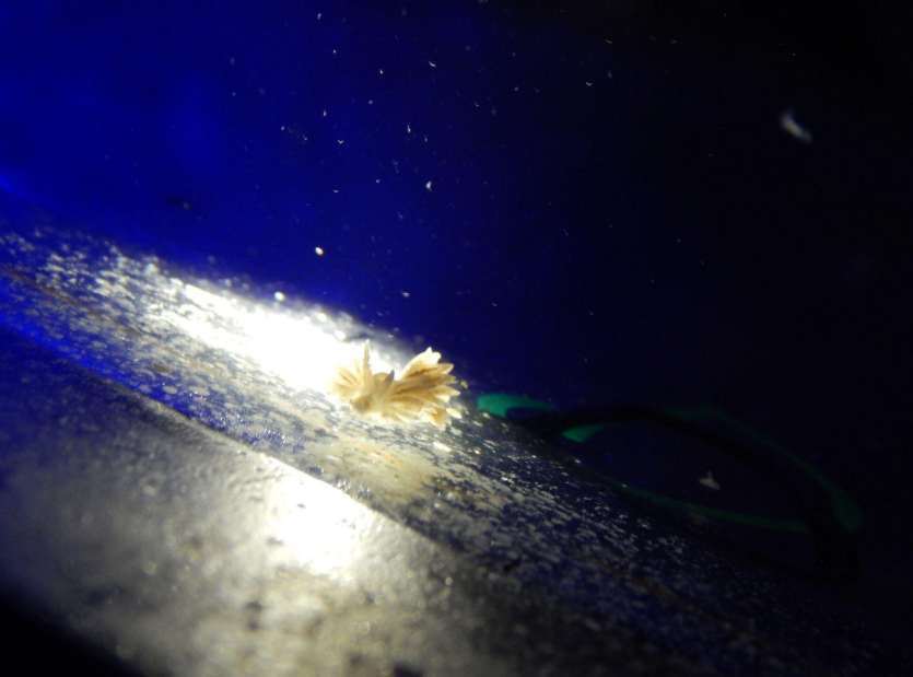
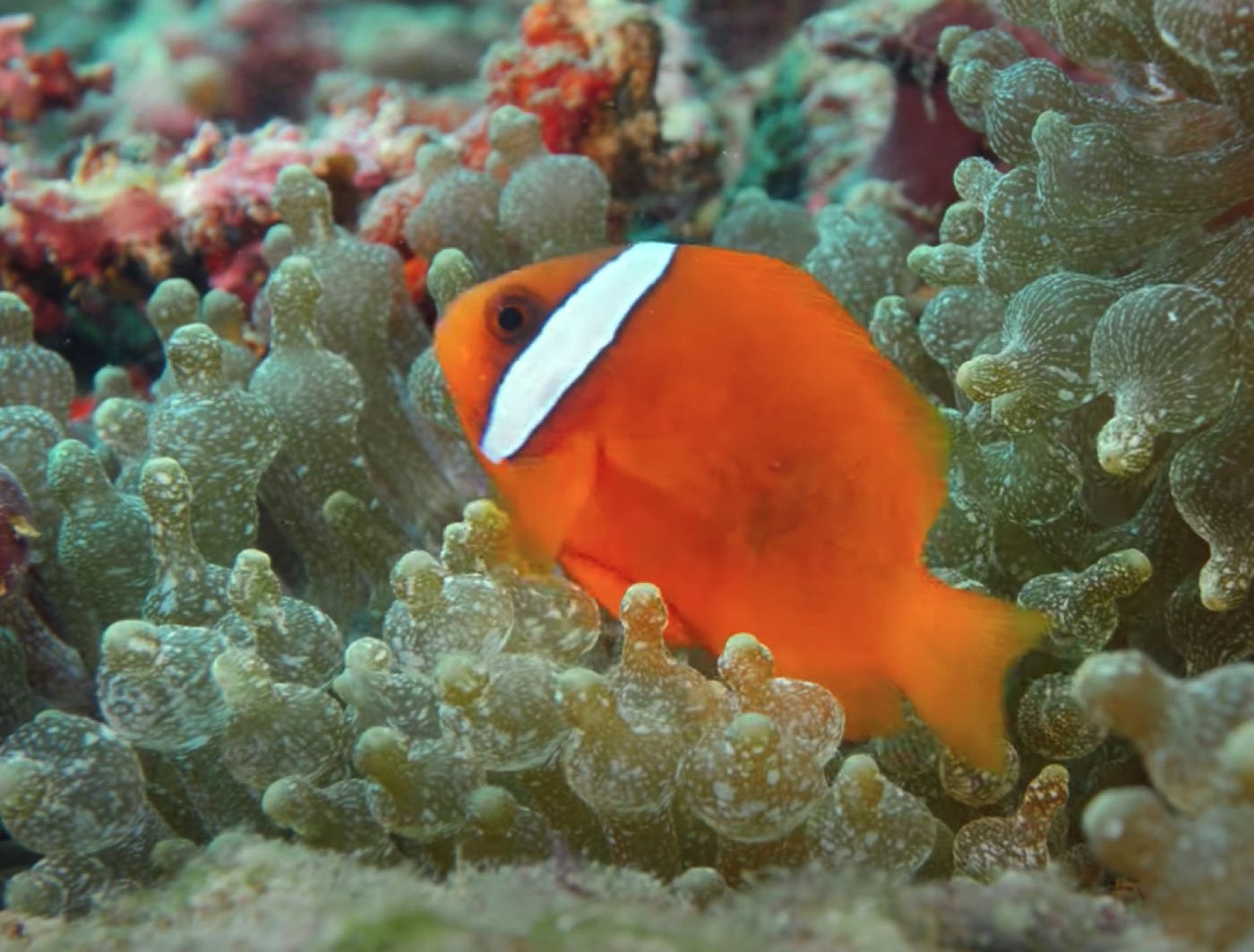
AN
ENGINEERING VIEW OF AQUARIUM SYSTEMS DESIGN: PUMPS AND PLUMBING
by
SANJAY JOSHI, Ph.D., NATHAN PADEN & SHANE GRABER
Sponsored in part by:
Every
aquarist at one time or another has had to deal with plumbing issues
such as sizing of pumps, selecting pipe size, determining whether the
pump can be upgraded without changing the returns in the overflow box,
maintaining water flow while controlling velocity so that it does not
blow off the coral tissue, etc.
A
lot of this information is available in the form of “rules of thumb”
as well as established fluids engineering formulas and data.This is an attempt to explain the basics of the devices used to
create and manage water flow and to provide a better understanding of
the principles involved as well as trying to consolidate the relevant
information for an aquarist in one single document.
In
addition to providing the theory, formulas and tables of relevant data,
for practical use we also provide an Excel
spreadsheet that incorporates all the useful information in a
useable form, without the requirement that the user understand the math
and formulas needed for solving the plumbing design problems.
Pump
Basics
Pumps
are the most common devices used to move water through the filters,
skimmers, and create circulation in the tanks.The most common type of pump used is called the centrifugal pump.The centrifugal pump is basically a rotary machine and comprises
3 main elements.
The
impeller - rotating element
The
volute- the casing inside which the impeller rotates
The
motor - imparts the rotation to the impeller
Proud sponsor of this column
The
pump functions by converting the rotational energy of the motor to
kinetic energy of the liquid by accelerating the liquid from the
center of the impeller to the outer via centrifugal force.The amount of energy imparted depends on the velocity of
the liquid at the tip of the impeller.Similar to rotating an object tied to a string, the velocity
will be higher if the speed of rotation is higher or the diameter
of the impeller is larger. The volute of the pump harnesses this
kinetic energy by creating a resistance to the flow and slowing it
down, this results in the creation of pressure energy.So in reality a centrifugal pump only creates flow, and the
resistance to this flow is what creates the pressure. Flow is
typically measured in GPH (Gallons per Hour) or GPM (Gallons per
Minute).
The
impeller is driven by a motor and is usually connected to the
motor in 2 ways. Direct coupling to the motor via a shaft –
called direct drive pumps,magnetically
coupled.
Pumps
with the impellers directly connected to the motor via the shaft require
the use of a mechanical seal, which are prone to failure and end up with
leaks. The magnetic coupled pumps avoid the seal problem by using
magnets to drive the impeller, thus allowing the creation of a
centrifugal pump that does not require a mechanical seal. For reef
aquarium applications the best choice is typically the magnetically
driven centrifugal pump and most of the common brands are of this
design.
The
kinetic energy that is created by the pump is often measured as head.Head refers to the height of a liquid column which the pump could
create using the kinetic energy that is generated by the pump.If the discharge of the pump is pointed straight up into the air,
it will pump the fluid to a certain height – the maximum head or shut
off head.This is usually determined by the speed of the motor and outside
diameter of the pumps impeller.
The
amount of fluid the pump moves is measured by the flow rate in GPH or
GPM. The flow rate can be converted to velocity of fluid as follows:
(1)
Velocity
= feet/sec
GPM
= Gallons per Min
D
= Inside diameter of pipe in inches
From
this we can see the first important observation about velocity and pipe
diameter.Doubling the pipe diameter will decrease the velocity by a factor
of 4.
Pumps
are rated by flow rate, head, and power consumption.When designing an aquarium system we are concerned with X amount
of flow at Y amount of head.Each pump will have its own relationship between head and flow
rate, depending on the pump design, and this information will typically
be displayed on the pump performance curve. For any pump, the flow rate
will reduce as the amount of head increases.
Pipes
and Piping Systems
The
flow of the pump is channeled through pipes and the piping system
comprising the pipes, fittings, control valves, etc.Solving fluid flow problems requires the use of a few basic
equations. The first one is the simple law of conservation of mass,
where the flow rate between any 2 sections is conserved.
(2)
The
second is the energy equation between any 2 sections of a pressurized
pipe. The energy equation between any two sections of a pressurized pipe
can be written as
(3)
Where:Z = elevation of centerline of pipe relative to an arbitrary
datum
P
= pressure on centerline of pipe
γ
= Specific Weight of Fluid
V
= average flow velocity
Hf
= head loss due to friction
Hm
= minor losses
As
the water flows through the pipe and piping system it encounters
resistance, primarily due to the following 3 elements: resistance
due to the elevation it has to raise the water – called static
head, or static head loss resistance due to friction with the walls
of the pipe – friction loss resistance due to the fittings and
valves used in the piping system.
The
cumulative effect of this resistance is to reduce the resulting flow
at the outlet. This cumulative resistance is often measured in terms
of head or pressure loss, and also called the total dynamic head (TDH)
of the piping systems.
To
determine the flow parameters at the outlet we need to compute the
TDH.Let us look at each one of the components separately:
Proud sponsor of this column
Resistance
due to elevation – Static Head
The
pump is used to move the liquid from a lower point to a higher point.The difference between the height of the liquid levels at the
output and input of the pump is the static head.
Friction
Loss in Pipes
As
the fluid flows through the pipe, friction on the side walls of the pipe
create resistance to the flow.Two
approaches are used to estimate the friction loss:
Using
published tables
Using
the governing equations
1)
Using Published Tables
Tables
indicating friction loss are available at several web sites, one such
table is published below as Table 1.These tables are typically derived using the empirical formula
called the Hazen-Williams formula. This formula is as follows:
(4)
Where:Hf = Friction loss in feet of head
L
= Length of pipe in feet
Q
= flow rate in GPM
D
= Nominal pipe ID in inches
C
= friction factor from Hazen-Williams
The
value of C is critical for computation and relates to the roughness of
the interiorwall of the pipe. One of the reasons that you find that tables
are not identical is due to the fact that different values of C are used
for the same material. For PVC pipe the value of C ranges from 140 to
150.
The
Hazen Williams formula has a limited range of validity and is only valid
for turbulent flow with reasonable velocity [Ref. C.P. Liou]. However,
for the range of typical values in a reef aquarium the formula is quite
valid.
Table
1: A Published Table for Friction loss in Schedule 40 PVC
Friction
Loss Per 100 Feet of SCH 40 Plastic Pipe
Nominal Pipe Diameter
GPM
1/2"
3/4"
1"
1 1/4"
1 1/2"
2"
3"
4"
1
2.08
0.51
-
-
-
-
-
-
2
4.16
1.02
0.55
0.14
0.07
-
-
-
5
23.44
5.73
1.72
0.44
0.22
0.066
0.015
-
7
43.06
10.52
3.17
0.81
0.38
0.11
0.021
-
10
82.02
20.04
6.02
1.55
0.72
0.21
0.03
-
15
-
42.46
12.77
3.28
1.53
0.45
0.07
-
20
-
72.34
21.75
5.59
2.61
0.76
0.11
0.03
25
-
-
32.88
8.45
3.95
1.15
0.17
0.04
30
-
-
46.08
11.85
5.53
1.62
0.23
0.06
35
-
-
-
15.76
7.36
2.15
0.31
0.08
40
-
-
-
20.18
9.43
2.75
0.41
0.11
45
-
-
-
25.1
11.73
3.43
0.51
0.17
50
-
-
-
30.51
14.25
4.16
0.61
0.16
60
-
-
-
-
19.98
5.84
0.85
0.22
70
-
-
-
-
-
7.76
1.13
0.31
75
-
-
-
-
-
8.82
1.28
0.34
80
-
-
-
-
-
9.94
1.44
0.38
90
-
-
-
-
-
12.37
1.8
0.47
100
-
-
-
-
-
15.03
2.18
0.58
2)
Using the Governing Equations
This
approach is based on using the Darcy-Wiesenbach equation and is valid
for all types of flow. This approach is the one most commonly used in
software packages for fluid flow analysis. The Darcy-Weisbach method is
generally considered more accurate than the Hazen-Williams method.Additionally, the Darcy-Weisbach method is valid for any liquid
or gas; Hazen-Williams is only valid for water at ordinary temperatures
(40 to 75o F).The Hazen-Williams method is very popular, especially among civil
engineers, since its friction coefficient (C) is not a function of
velocity or pipe diameter.Hazen-Williams is simpler than Darcy-Weisbach for calculations
where you are solving for flowrate, velocity, or diameter.
The
main governing equation for friction loss is Darcy’s equation
(5)
Where:Hf = friction loss in feet of head
f = dimensionless friction factor
L = Pipe Length in FEET
D = Pipe Inside Diameter in FEET
V = Flow Velocity in FEET PER SECOND
g = Gravitational Constant = 32.2 feet per second squared
From
this equation it is quite clear that the flow velocity has a big impact
on frictional losses. From equation 1 we know that the flow velocity is
inversely proportional to the square of the pipe diameter. So if we
reduce the pipe diameter by ˝, we increase the flow velocity by a
factor of 4 and hence also increase the friction loss by a factor of 16.
To
apply this equation we need to determine the friction factor f, which is
the complicated part.The
steps are as follows:
We
first need to determine the type of flow which is typically determined
from the Reynold’s number, which rates the type of flow in the pipe:
Laminar, Turbulent or Transitional flow.The Reynold’s number is a dimensionless number and is
calculated as follows
(6)
D=
diameter of pipe in Feet
V
= velocity in Feet/sec
= kinematic viscosity of
the fluid being pumped
The
kinematic viscosity is the ratio of the fluid’s density and the fluids
absolute viscosity. The kinematic viscosity changes according to
temperature, see table (www.pump.net)
Table
2 : Kinematic Viscosity of Fresh Water
Temp
(degrees F)
Kinematic
Viscosity of fresh water
70
1.0265
x 10-5 ft2/sec
75
9.6199
x 10-6 ft2/sec
80
9.0363
x 10-6 ft2/sec
Kinematic
Viscosity is the ratio of the fluid's density and the fluid's absolute
viscosity. These values are for FRESH water. For saltwater multiply the
kinematic viscosity of water by 1.024 (or whatever your planned specific
gravity will be).
This
Reynolds Number will tell us whether a particular flow is laminar, in
the transition zone, or is turbulent, and the following chart gives the
generally accepted ranges for these flows:
Table
3: Relationship between Reynolds Number and Type of Flow
Reynolds
Number
Flow
Type
RD
< 2300
Laminar
2300
< RD < 4000
Transitional
4000
< RD
Turbulent
For
most of our application the flow through the pipes will generally be
turbulent.
Once
the type of flow is determined, the next step is to calculate the
friction factor.
The
Moody Equation is used to calculate the dimensionless friction factor f.
and originates from a paper published by Lewis F. Moody in 1944.Typically the values can be read off a Moody diagram (see http://www.mestudent.com/fluids/moody.htm
for a Moody Chart) which is created using the Colebrook-White formula
(7)
Where:f is the friction factor
ε
= roughness factor (generally .000005 ft for PVC pipe.)
D
= diameter in inches
Re
= Reynold’s number
The
equation is difficult to solve in close form since f appears on both
sides of the equation.It has to be solved numerically.
The
Swamee-Jain approximation can be used to calculate the friction factor
under certain conditions (where ε/D < .02 and Re >
3000),and
gives results within 3% of the results obtained from the Moody diagram.
It has the advantage of being easily programmed in a computer or
calculator. For most of the aquarium applications the flow is turbulent.
The Swamee-Jain approximation for the friction factor is as follows: